Open Journal of Statistics
Vol.04 No.08(2014), Article ID:49939,10 pages
10.4236/ojs.2014.48055
A Multivariate Test for Three-Factor Interaction in 3-Way Contingency Table under the Multiplicative Model
Njoku O. Ama
Department of Statistics, University of Botswana, Gaborone, Botswana
Email: njoku52@gmail.com, amano@mopipi.ub.bw
Copyright © 2014 by author and Scientific Research Publishing Inc.
This work is licensed under the Creative Commons Attribution International License (CC BY).
http://creativecommons.org/licenses/by/4.0/


Received 16 June 2014; revised 22 July 2014; accepted 30 July 2014
ABSTRACT
Two test statistics that have been commonly used in analysing interactions in contingency table are the Pearson’s Chi-square statistic, χ2, and likelihood ratio test statistic, G2. Both test statistics, in tables with sufficiently large sample size, have an asymptotic chi-square distribution with degrees of freedom (df) equal to the number of free parameters in the saturated model. For example under the hypothesis of independence of the row and column conditioned on the layer in an I × J × K contingency table, the df is K(I − 1)(J − 1). These test statistics, in large sized tables, will have less power since they have large degrees of freedom. This paper proposes a product effect model, which combines the advantages of the multiplicative models over the additive, for analysing the interaction between the row and column of the 3-way table conditioned on the layer. The derived statistics is shown to be asymptotically chi-square with a small degree of freedom, K − 1, for the I × J × K contingency table. The performance of the developed statistic is compared with the Pearson’s chi-square statistic and the likelihood ratio statistic test using an illustrative example. The results show that the product effect test can detect interaction even when some of the main effects are not significant and can perform better than the other competitors having smaller degree of freedom in large sized tables.
Keywords:
Contingency Tables, Product Effect, Models, Interaction

1. Introduction
A 3-way contingency table is a cross-classification of observations by the levels of three categorical variables—A, B, and C. The levels can be ordinal or nominal. If n units in a sample are independently and identically distributed (IID); that is, if they constitute a random sample, then the vector of cell counts
 has a multinomial distribution with index
 and a parameter,
 , where
 probability that a randomly selected unit falls into the
 cell of the contingency table with variables A, B and C. The probability distribution
 is the joint distribution of A, B, and C.
Interaction in the 3-way contingency has been tested using the chi-square statistic and the likelihood ratio test statistic with
 degree of freedom [1] -[3] . Grizzle et al. [4] , Darroch [5] and Johnson and Graybill [6] have modelled interaction as a product of the marginal effects or components of the ways of classification of the table. Tukey [7] in order to overcome the difficulty in testing for interaction in the two-factorial experiment with one observation per cell modelled the two-factor interaction as a product of the effects of the two factors and developed a one degree of freedom F-test for analysing the interaction between the factors. Drawing an analogy from the two factorial experiments we can view the 2-way contingency table as a two-factorial experiment with one observation per cell similar to the Poisson modelling of 2-way contingency table where the cell observations are seen as the mean number of occurrences of the event within a defined infinitesimal interval. The I × J × K contingency table can be viewed as K 2-way contingency table. The present paper argues that the transformation of the contingency table applicable in the likelihood ratio tests [1] [8] is often unnecessary but that the data can be analysed in a manner similar to the Pearson’s chi-square which does not transform the data. A multivariate approach is adopted in analysing the interaction in an I × J × K table, under the product effect model, where the three-factor interaction is defined as a product of the effects of the ways of classification of the table. The advantage of the proposed model is that it gives rise to chi-square tests with smaller degrees of freedom, irrespective of the size of the table, which is conjectured to have greater power than other tests with larger degrees of freedom. It has been shown [9] [10] that the power of the noncentral chi-square statistics, for a given value of non-centrality parameter and level of significance, increases as the degree of freedom decreases. Our results will be of some practical value to researchers who are involved in analysing mutual independence in higher order tables as their results will be based on small degrees of freedom leaving extra degrees of freedom for further decomposition of other forms of independence in the data. Extension of the proposed method to higher order tables is straightforward.
Model for 3-Factor Interaction
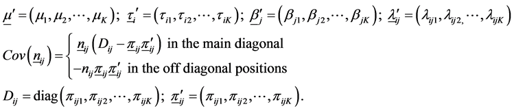
Let us assume that we have an I × J × K 3-way contingency, representing respectively the row, column and layer classifications of the table, and that the K-dimensional vector
 of frequency layers available in the
 cell has associated it with a K-dimensional vector
 of unknown cell probabilities such that
 . In addition if we assume that
 follows a multinomial probability distribution given by
 (1.1)
(1.1)
 is fixed,

 are independent for all

The 3-way contingency table under the multinomial structure described above is similar to the layout of a three-factorial experiment with one observation per cell. In the spirit of [7] and drawing an analogy from the factorial experimental structure, a linear additive model for the observed cell probability in the
 -cell can be written as in (1.2). The interest is in the consideration of models where these probabilities depend on a vector
 of covariates associated with the
 individual or group.
Under the assumption (1.1), and given the
 layer, we have an identity relation
 (1.2)
(1.2)
where,
 ,
,
 and
and
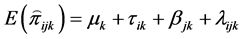
 denote respectively the overall probability for the kth layer, ith row, and jth column for the kth layer. Reasoning by analogy from the regular analysis of variance, we get a linear additive model for (1.2) as
 (1.3)
(1.3)
where,
 is the overall probability of an observation belonging to the kth layer of the 3-way contingency table;
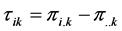 is the effect of the ith row of the table for the kth layer;
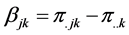 is the effect of the jth column of the table for the kth layer;
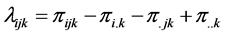 is the interaction between the ith row and jth column for the kth layer of the table. These parameters are subject to the restrictions:
 (1.4)
(1.4)
and are independent of the kth layer.
The relation (1.3) can be recast in vector notation as
 (1.5)
(1.5)
Or
 (1.6)
(1.6)
where,
 (1.7)
(1.7)
Estimation of the parameters of this model (1.6) by maximum likelihood proceeds by maximization of the multinomial likelihood (1.1) with the probabilities
 viewed as functions of the parameters
 ,
,
 ,
,
 , and
, and
 in the Equation (1.3) and yields
 (1.8)
(1.8)
where,
The matrix
 is given as

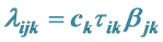
For the kth layer, the interaction between the ith row and jth column is defined multiplicatively as being proportional to the ith row effect and jth column effect and given as
 (1.9)
(1.9)
where, ck is an unknown constant for the layer;
 and
and
 are respectively the effect of the ith row and jth column for the kth layer. The model (1.9) is referred to as the product effect model [2] [3] . The classical method of partitioning the chi-squares for the 3-way
 contingency table does not provide a convenient test of the null hypothesis that the 3-way interaction is zero [11] . The model indicates that the three-factor interaction in the contingency table and for the kth layer response is proportional to the product of the effects of ith row classification and the jth column classification of the table. Darroch [12] has demonstrated the advantages of the multiplicative interaction models over the additive.
2. Development of Test Statistics Based on the Model
Rewriting (1.9), the model for the two-factor interaction for the kth layer response, in vector notation,
 (2.1)
(2.1)
where

The matrix of interaction
 can be written as
 (2.2)
(2.2)
From (1.5) or (1.6) the residual after substituting (2.1) becomes
 (2.3)
(2.3)
 (2.4)
(2.4)

This gives the least square estimate
 of
of
 as
as
 (2.5)
(2.5)
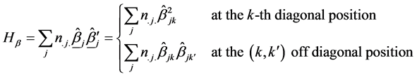
The matrix of sum of squares sum of product (SS-SP) for interaction from (2.3) is
 (2.6)
(2.6)
with expectation
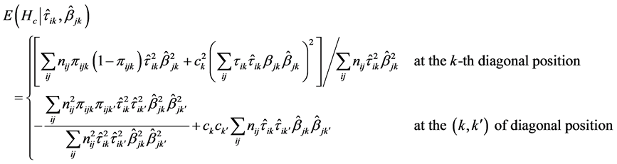 (2.7)
(2.7)
The total sum of squares and cross product (SS-SP) is given as
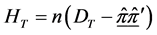 (2.8)
(2.8)
where,
 (2.9)
(2.9)
The expectation of
 is
is

 (2.10)
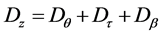
The total SS-SP matrix
 can be partitioned into unit SS-SP,
 , SS-SP due to the row effect,
 , SS-SP due to the column effect,
 , and SS-SP due to the residual,
 , namely
 (2.11)
The unit SS-SP matrix
 is given by
 (2.12)
with
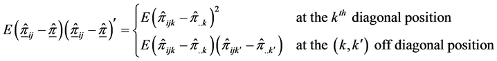
The expectation of
 is given by
 (2.13)
The matrix of SS-SP for the row effect,
 , is
, is
 (2.14)
With expectation,
 (2.15)
 and
and
 (2.16)

The matrix of SS-SP,
 , due to the column effect is
 (2.17)
With expectation,
 (2.18)

and
 (2.19)
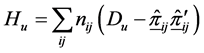
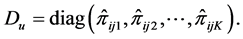
The matrix of SS-SP for the residual (2.3) is
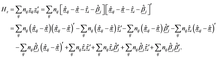 (2.20)
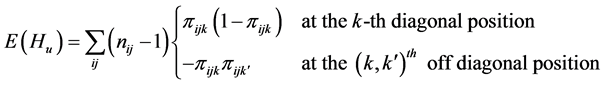
With expectation
 (2.21)
Since the cross-product terms will vanish on taking expectation because of independence and restriction in (1.4)
 (2.22)
Hence,
 (2.23)
where,
 (2.24)
and

 , with
 (2.25)
The hypothesis of no interaction,
 , for all k, implies that either
 or
or
 or
or
 for all k.
Hence
 . (2.26)
Under the null hypothesis (2.26), in which case , and reasoning from (2.13) for the
 layer,

Similarly, ;
;
 (see Section 1.1)
 (2.27)
However, whether or not
 is true,

where V is as defined in (2.10). Each of the quantities ,
,
 ,
,
 ,
,
 ,
,
 and
and
 provides an estimate of V and can be employed in the construction of tests of significance of the row, column effects and interaction provided that they are independent.
Independence of HT, Hc, Hτ, Hβ
By appealing to the following theorem [13] , it can be shown that the quadratic forms HT, Hc, Hτ and Hβ, are independent.
Theorem 2.1. Let
 be distributed
 , the set of positive semi-definite quadratic forms
 ,
,
 ,
,
 ,
,
 are jointly independent if and only if
 , the null matrix for all
 .
.
Theorem 2.2. As , the matrices
 ,
,
 ,
,
 and
and
 are independent.
By theorem 1, the joint independence of HT, Hc, Hτ and Hβ implies pairwise independence.
3. Construction of Test Statistic for the Hypothesis
Recall that
 follows
 . As
. As
 tends to a constant, say
 , then
 will follow asymptotic
multivariate normal distribution with mean
 and variance,
 , where
 is a singular matrix given by (1.7). Therefore
 has a singular normal distribution.
Under the hypothesis,
 , the matrix Hc has a pseudo Wishart distribution with parameter 1 and
 . The random matrix HT follows the Wishart distribution with parameter
 and V and inde-
pendent of Hc. They can be used in constructing the determinant based test statistic for the hypothesis

Since the matrix V is nonsingular, by generating the matrix of contrasts, say B and pre- and post-multiplying each of them by B and B transpose, V can be made non-singular.
Let
 (3.1)
(3.1)
 is an
is an
 column vector of independent variables for the kth response. Also define
 such that
Then
 (3.2)
(3.2)
where
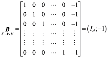 (3.3)
(3.3)
The matrix B is of full rank,
 and
and
 is a
is a
 identity matrix.
Certainly,
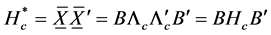 (3.4)
(3.4)
is a non-singular transformation of the matrix Hc and so also is the matrix
 (3.5)
(3.5)
The hypothesis

is similarly transformed to
 or
or 
However, [14] and [15] have discussed the equivalence between
 and
and
 and the invariant property of the Wilks
 criterion under such transformation as above. Also the quadratic forms
 and
and
 (3.4 and 3.5) are independent Wishart distributed matrices with same degrees of freedom as
 and
and
 respectively and variance-covariance matrix
 . Hence the analogue of the Wilks criterion can be used in testing the hypotheses and is given by
 (3.6)
(3.6)
where
 defines the Wilks distribution with parameters
 . It has been shown (see e.g. Kshirsagar, 1972) that
 (3.7)
(3.7)
where
 is the square of the ith sample canonical correlation and the root of the determinantal equation
 (3.8)
(3.8)
and
 is related to
 the root of the determinantal equation
 (3.9)
(3.9)
by the relation
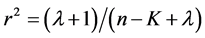 (3.10)
Under the null hypothesis,
 and using (3.9), that is
 ,
, .
.
It has been shown, [16] , that

where , using the notation in this paper.
Thus,
 (3.11)
under .
.
Asymptotically as ,
,
 (3.12)
Hence
 (3.13)
The best value of m for the expectation on both sides of (3.13) to be equal is .
.
Therefore,
 (3.14)
and can provide a test criterion for the rejection or non-rejection of .
.
The test rejects the hull hypothesis if
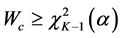 at an
at an
 -level of significance.
4. Illustrative Example
The application of the developed test makes use of data taken from [17] (see Table 1). The data represent the attitude of 333 undergraduate students of University of Nigeria towards taking up teaching as a profession after graduation. The students were sampled from three groups of faculties,
 ,
,
 and
and . The responses Y (yes), N (no), U (undecided) indicates willing, not willing and undecided respectively.
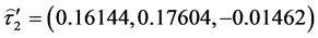
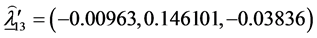
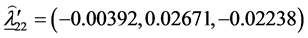
The estimates of the parameters in (1.5) are:
 ;
; ;
; ;
; ;
; ;
;
 ;
; ;
;
 ;
; ;
;
 ;
; ;
;
 ;
;
The matrix of SS-SP due to interaction,
 , is
, is
 ;
;
Therefore,
 ;
; ;
;
 ;
; ;
;
 ;
;
Similarly,


These values are summarized in the Table 2.

Table 1. Attitude of university students towards the teaching profession.
Table 2. Multanova of categorical data for attitude of students towards teaching.
m = 330.
The Pearson’s chi-square for testing the hypothesis of no interaction (independence of the row and column for the kth response),
 gives the computed value of the test statistic as, X2 = 8.214 based on 6 d.f while the likelihood ratio test statistic, G2 for testing H0 is calculated as G2 = 7.804. Both test statistics are based on 6 degrees of freedom and show that interaction is not significant.
5. Conclusion
The results of the analysis show that while the effect of the sex and interaction are significant in the data, the effect of faculty is not significant. Thus, the proposed test for interaction based on the product effect model and based on 2 degrees of freedom
 can produce significant results even when one of the factors in the interaction is not significant. The test performs better than the traditional tests—the Pearson’s chi square and the likelihood ratio tests, and could still out perform them in having greater power in larger 3-way contingency tables since it will have smaller degree of freedom. [9] has shown that the power of the non-central chi-square test at a given level of significance and non-centrality parameter increases as the degree of freedom decreases.
References
- Cheng, P.E., Liou, M. and Aston, J.A.D. (2009) Likelihood Ratio Tests with Three-Way Tables. Institute of Statistical Science, Academia Sinica 2CRiSM, Department of Statistics, The University of Warwick, UK. http://www3.stat.sinica.edu.tw/library/c_tec_rep/2007-3-20090206.pdf
- Agresti, A. (2002) Categorical Data Analysis. 2nd Edition, John Wiley and Sons Inc., Hoboken, 132. http://dx.doi.org/10.1002/0471249688
- Christensen, R. (1997) Loglinear Models and Logistic Regression. 2nd Edition, Springer-Verlag, New York Inc., New York.
- Grizzle, J.E., Starmer, F. and Koch, G.G. (1969) Analysis of Categorical Data by Linear Models. Biometrics, 25, 489- 504. http://dx.doi.org/10.2307/2528901
- Darroch, J.N. (1962) Interactions in Multi-Factor Contingency Tables. Journal of the Royal Statistical Society, B24, 251-263.
- Johnson, D.E. and Graybill, F.A. (1972) An Analysis of a Two-Way Model with Interaction and No Replication. Journal of the American Statistical Association, 67, 862-868. http://dx.doi.org/10.1080/01621459.1972.10481307
- Tukey, T.W. (1949) One Degree of Freedom for Non-Additivity. Biometrics, 5, 232-242. http://dx.doi.org/10.2307/3001938
- Cheng, P.E., Liou, M. and Aston, J.A.D. (2010) Likelihood Ratio Tests with Three-Way Tables. Journal of the American Statistical Association, 105, 740-749. http://dx.doi.org/10.1198/jasa.2010.tm09061
- Ama, N.O. (1991) On Multiplicative Models for Interaction in Contingency Tables. Unpublished Ph.D. Thesis, University of Nigeria, Nsukka.
- Hélie, S. (2007) Understanding Statistical Power Using Noncentral Probability Distributions: Chi-Squared, G-Squared, and ANOVA. Tutorials in Quantitative Methods for Psychology, 3, 63-69.
- Lancaster, H.O. (1969) The Chi-Squared Distribution. Wiley & Sons, Inc., New York.
- Darroch, J.N. (1974) Multiplicative and Additive Interaction in Contingency Tables. Biometrika, 61, 207-214. http://dx.doi.org/10.1093/biomet/61.1.207
- Graybill, F.A. (1961) An Introduction to Linear Statistical Models. McGraw-Hill, New York.
- Mardia, K.V., Kent, J.T. and Bibby, J.M. (1979) Multivariate Analysis. Academic Press, London.
- Kshirsagar, A.M. (1972) Multivariate Analysis. Marcel Dekker, Inc., New York.
- Bartlett, M.S. (1938) Further Aspects of the Theory of Multiple Regression. Mathematical Proceedings of the Cambridge Philosophical Society, 34, 33-40. http://dx.doi.org/10.1017/S0305004100019897
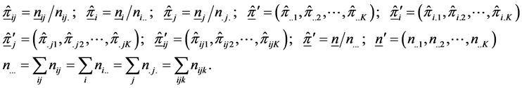
- Onukogu, I.B. (1985) An Analysis of Variance of Nominal Data. Statistica, anno, XLIV, No. 1, 87-96.