Open Journal of Statistics
Vol.3 No.3(2013), Article ID:33231,12 pages DOI:10.4236/ojs.2013.33021
Time Series Forecasting Using Wavelet-Least Squares Support Vector Machines and Wavelet Regression Models for Monthly Stream Flow Data
Faculty of Science, Department of Mathematics, Universiti Teknologi Malaysia, Skudai, Malaysia
Email: pandhiani@hotmail.com, ani@utm.my
Copyright © 2013 Siraj Muhammed Pandhiani, Ani Bin Shabri. This is an open access article distributed under the Creative Commons Attribution License, which permits unrestricted use, distribution, and reproduction in any medium, provided the original work is properly cited.
Received March 24, 2013; revised April 25, 2013; accepted May 2, 2013
Keywords: River Flow; Time Series; Least Square Support Machines; Wavelet
ABSTRACT
This study explores the least square support vector and wavelet technique (WLSSVM) in the monthly stream flow forecasting. This is a new hybrid technique. The 30 days periodic predicting statistics used in this study are derived from the subjection of this model to the river flow data of the Jhelum and Chenab rivers. The root mean square error (RMSE), mean absolute error (RME) and correlation (R) statistics are used for evaluating the accuracy of the WLSSVM and WR models. The accuracy of the WLSSVM model is compared with LSSVM, WR and LR models. The two rivers surveyed are in the Republic of Pakistan and cover an area encompassing 39,200 km2 for the Jhelum River and 67,515 km2 for the Chenab River. Using discrete wavelets, the observed data has been decomposed into sub-series. These have then appropriately been used as inputs in the least square support vector machines for forecasting the hydrological variables. The resultant observation from this comparison indicates the WLSSVM is more accurate than the LSSVM, WR and LR models in river flow forecasting.
1. Introduction
Pakistan is the home to the world’s largest contiguous irrigation system. This is an economy that is largely dependent on the agricultural sector; therefore, it has a vast irrigation network. The dependence on this form of farming is developed by a persistent rainfall pattern that keeps the rivers flowing, which in turn leads to the availability of irrigation waters flowing downstream. The Jhelum and Chenab rivers provide the biggest percentage of irrigation waters in various provinces in Pakistan.
These days, river flow forecasting has a major role to play in water resources system planning. The sources of water with many activities such as planning and operating system component estimate for future demand. The composition of water is necessary for both short-term and long-term forecasts of the event flow to optimize system or an application for the growth or decline in the future. There are many mathematical models to predict future flow of rivers such as discussed by [1-4].
The Support Vector Machine (SVM) [5] forecasting method has been used in various studies of hydrology water modeling and water resource processed such as flood stage forecasting [6], rainfall runoff modeling [7-9] and stream flow forecasting [10-12]. Researcher solved the standard SVM models using the complicated computational programming techniques, which are very expensive in time to handle the required optimization programming.
The Suykens and Vandewalls [13] proposed the least square support vector machines (LSSVM) model to simplify the SVM. In the various areas, such as regression problems and pattern recognition [14,15], the LSSVM model has been used successfully. LSSVM and SVM have almost similar advantages but the LSSVM has an additional advantage, e.g. it needs to solve only a linear system of equation, which is much easier to solve and predict results [1-4]. The LSSVM and SVM mathematical models have been used in predicting ad analyzing the future flow of rivers.
Recently, wavelet theory has been introduced in the field of hydrology, [16-18]. Wavelet analysis has recently been identified as a useful tool for describing both rainfall and runoff time series [16,19]. In this regard there has been a sustained explosion of interest in wavelet in many diverse fields of study such as science and engineering. During the last couple of decades, wavelet transform (WT) analysis has become an ideal tool studying of a measured non-stationary times series, through the hydrological process.
An initial interest in the study of wavelets was developed by [20-22]. Daubechies [22] employed the wavelets technique for signal transmission applications in the electronics engineering. Foufoula Georgiou and Kumar [23] used geophysical applications. Subsequently, [17] attempted to apply wavelet transformation to daily river discharge records to quantify stream flow variability. The wavelet analysis, which is analogous to Fourier analysis is used to decomposes a signal by linear filtering into components of various frequencies and then to reconstruct it into various frequency resolutions. Rao and Bopardikar [24] described the decomposition of a signal using a Haar wavelet technique, which is a very simple wavelet.
Wavelet spectrum, based on the continuous wavelet transform, has been proven to be a natural extension of the much more familiar conventional Fourier spectrum analysis which is usually associated with hydro metrological time series analysis [25]. Instead of the results being presented in a plot of energy vis a vis frequency for energy spectrum in Fourier Transform (FT) as well as FFT (Fast Fourier Transform), the wavelet spectrum is three dimensional and is plotted in the time frequency domain in which the energy is portrayed as contours. The wavelets are mathematical functions that break up a signal into different frequency components so that they are studied at different resolutions or scales. They are considered better than the Fourier analysis for their distinct signals that pose discontinuities and sharp spikes.
The main purpose of the this study is to investigate the performance of the WLSSVM model for streamflow forecasting and to compare it with the performance of the least square support vector machines (LSSVM), linear regression (LR) and wavelet regression models (WR).
2. Methods and Materials
2.1. The Least Square Vector Machines Model
LSSVM is a new version of SVM modified by [13]. LSSVM involves the solution of a quadratic optimization problem with a least squares loss function and equality constraints instead of inequality constraints. In this section, we briefly introduce the basic theory LSSVM in time series forecasting. Consider a training sample set  with input
  and output
 . In feature space SVM models take the form
 (1)
(1)
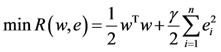
where the nonlinear mapping  maps the input data into a higher dimensional feature space. LSSVM introduces a least square version to SVM regression by formulating the regression problem as
 (2)
(2)
subject to the equality constraints
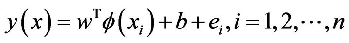 (3)
(3)
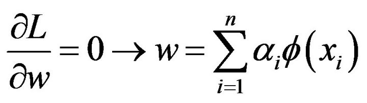
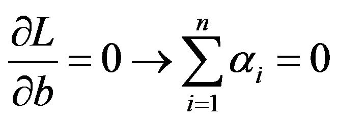
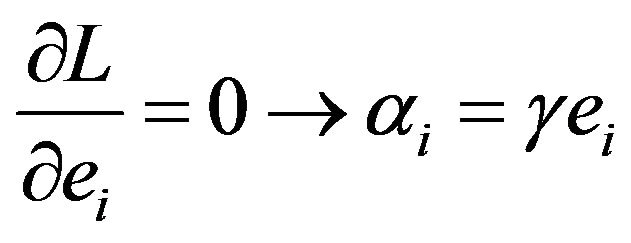
To solve this optimization problem, Lagrange function is constructed as
 (4)
(4)
where,  is Lagrange multipliers. The solution of (6) can be obtained by partially differentiating with respect to
  and
and 
 (5)
(5)
 (6)
(6)
 (7)
(7)
 (8)
(8)
then the weight w can be written as combination of the Lagrange multipliers with the corresponding data training .
.
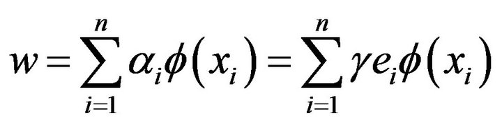 (9)
(9)
If we put the result of Equation (9) into Equation (3), then the following result is obtained:
 (10)
(10)
where, a positive definite kernel is defined as follows:
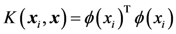 (11)
(11)
The ![]() vector and b can be found by solving a set of linear equations:
vector and b can be found by solving a set of linear equations:
 (12)
(12)
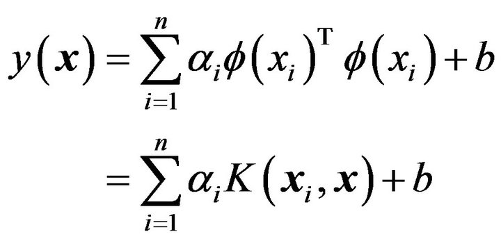
where, . This finally leads to the following LSSVM model for function estimation:
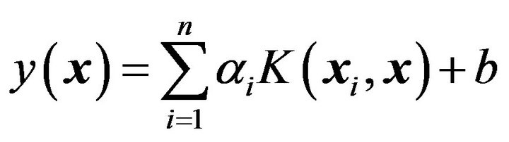 (13)
(13)
where ,
,  are the solution to the linear system. Kernel function,
 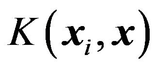 represents the high dimensional feature space that is nonlinearly mapped from input space x. The typical examples of the kernel function are as follows:
 (14)
(14)
Here  and
and ![]() are the kernel parameters. The architecture of LSSVM is shown in Figure 1.
are the kernel parameters. The architecture of LSSVM is shown in Figure 1.
2.2. Wavelet Analysis
Wavelets are becoming an increasingly important tool in time series forecasting. The basic objective of wavelet transformation is to analyze the time series data both in the time and frequency domain by decomposing the original time series in different frequency bands using wavelet functions. Unlike the Fourier transform, in which time series are analyzed using sine and cosine functions, wavelet transformations provide useful decomposition of original time series by capturing useful information on various decomposition levels.
Assuming a continuous time series , a wavelet function can be written as:
 (15)
(15)
where  stands for time,
 ![]() for the time step in which the window function is iterated, and
for the time step in which the window function is iterated, and  for the wavelet scale.
  called the mother wavelet can be defined as
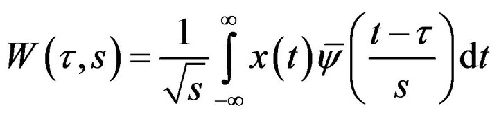
 . The continuous wavelet transform (CWT) is given by
 (16)
(16)
where  stands for the complex conjugation of
 .
.  presents the sum of over all time period
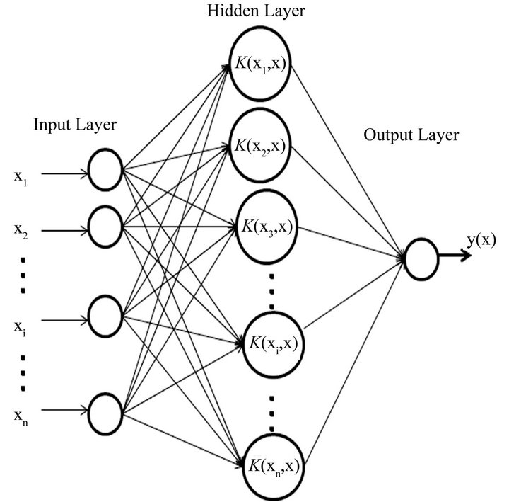
Figure 1. Architecture of LSSVM.
of the time series multiplied by scale and shifted version of wavelet function . The use of continuous wavelet transform for forecasting is not practically possible because calculating wavelet coefficient at every possible scale is time consuming and it generates a lot of data.
Therefore, discrete wavelet transformation (DWT) is preferred in most of the forecasting problems because of its simplicity and ability to compute with less time. The DWT involves choosing scales and position on powers of 2, so-called dyadic scales and translations, then the analysis will be much more efficient as well as more accurate. The main advantage of using the DWT is its robustness as it does not include any potentially erroneous assumption or parametric testing procedure [26-28]. The DWT can be defined as
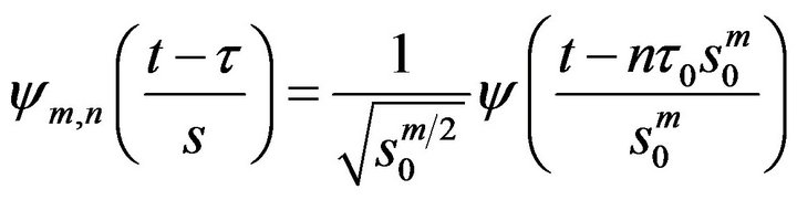 (17)
(17)
where m and n are integers that control the scale and time, respectively;  is a specified, fixed dilation step greater than 1; and
  is the location parameter, which must be greater than zero. The most common choices for the parameters
  and
and . For a discrete time series
  where
where  occurs at discrete time t, the DWT becomes
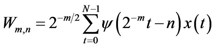 (18)
(18)
where ![]() is the wavelet coefficient for the discrete wavelet at scale
is the wavelet coefficient for the discrete wavelet at scale  and
and . In Equation (18),
  is time series
 , and N is an integer to the power of
 ; n is the time translation parameter, which changes in the ranges
 , where
 .
.
According to Mallat’s theory [20], the original discrete time series  can be decomposed into a series of linearity independent approximation and detail signals by using the inverse DWT. The inverse DWT is given by [20,26,27]
 (19)
(19)
or in a simple format as
 (20)
(20)
which  is called approximation sub-series or residual term at levels M and
  are detail sub-series which can capture small features of interpretational value in the data.
3. Study Area
The time series of monthly streamflow data of the Jhelum and Chenab river of Pakistan are used. The locations of the Jhelum and Chenab catchments are shown in Figure 2. The Jhelum River catchment covers an area of 21,359 km2 and the Chenab catchment covers 28,000 km2. The first set of data comprises of monthly streamflow data of Chanari station at Jhelum River from Jan 1970 to December 1996 and the second data of set of streamflow data of Marala station at Chenab River from April 1947 to March 2007. In the applications, the first 20 years and 51 year of flow Jhelum data and Chenab data (237 months and 430 months, 80% of the whole data set) were used for training the network to obtain the parameters model. Another dataset consisting of 75 monthly records (20% of the whole data) was used for testing.
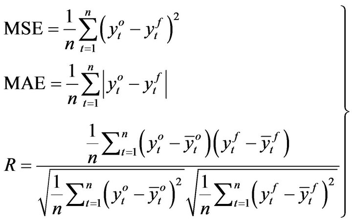
The performances of each model for both training and testing data are evaluated by using the mean-square error (MSE), mean absolute error (MAE) and correlation coefficient (R) which is widely used for evaluating results of time series forecasting. MSE, MAE and R are defined as
 (21)
(21)
where  and
and  are the observed and forecasted values at time
 , respectively and n is the number of data points. The criteria to judge for the best model are
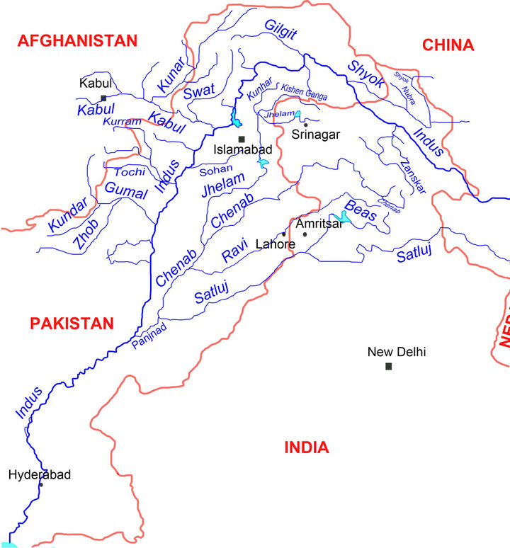
Figure 2. Location map of the study area.
relatively small of MAE and MSE in the training and testing. Correlation coefficient measures how well the flows predicted, correlate with the flows observed. Clearly, the R value close to unity indicates a satisfactory result, while a low value or close to zero implies an inadequate result.
4. Model Structures
One of the most important steps in developing a satisfactory forecasting model such as LSSVM and LR models is the selection of the input variables. The appropriate input variables will allow the network to successfully map the desired output and avoid loss of important information. There are no fixed rules in selection of input variables for developing this model, even though a general framework can be followed based on previous successful application in water resources problems [12,29, 30]. In this study, the six model structures were developed to investigate variable enabling of input variables on model performance. Six model structures are accomplished by setting the input variables equal to the number of the lagged variables from monthly stream flows of previous periods data,  , where p is set 1, 2, 3, 4, 5 and 6 months. The model structure for original and DWT monthly streamflow data can be mathematically expressed as

and
where  denotes the streamflow value of 1 previous month,
  is obtained by adding the effective Ds (D2, D4 and D8), and approximately components of the
  values. The model input structures for forecasting streamflow of Jehlum River and Chenab River is shown in Table 1.
5. Results and Discussion
5.1. Fitting LSSVM to the Data
The selection of appropriate input data sets is an important consideration in the LSSVM modeling. In the training and testing of LSSVM model, the same input structures of the data set (M1 - M6) were used. In order to obtain the optimal model parameters of the LSSVM, a grid search algorithm and cross-validation method was employed. Many work on the use of the LSSVM in time series modeling and forecasting have demonstrated favorable performances of the RBF [6,31,32]. Therefore, RBF is used as the kernel function for streamflow forecasting in this study. The LSSVM model used herein has two parameters  to be determined. The grid search method is a common method which was applied to calibrate these parameters more effectively and systematically to overcome the potential shortcomings of the trails and error method. It is a straightforward and exhaustive method to search parameters. In this study, a grid search of
  with
with  in the range 10 to 1000 and
  in the range 0.01 to 1.0 was conducted to find the optimal parameters. In order to avoid the danger of over fitting, the cross-validation scheme is used to calibrate the parameters. For each hyper parameter pair
  in the search space, 10-fold cross validation on the training set was performed to predict the prediction error. The best fit model structure for each model is determined according to the criteria of the performance evaluation.
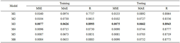
Tables 2(a) and 2(b) show the performance results obtained in the training and testing period of the regular LSSVM approach (i.e. those using original data). For the

Table 1. The model structures for forecasting streamflow of Jhelum and Chenab Rivers.
 (a)
(a)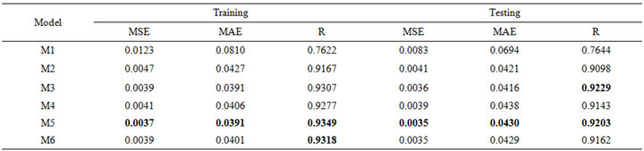 (b)
(b)
Table 2. Forecasting performance indicates of LSSVM for (a) Jhelum River of Pakistan; (b) Chenab River of Pakistan.
training and testing phase in Jehlum stations, the best values of the MSE, MAE and R were obtained using M3. In the model M3 had the smallest MAE and MSE whereas it had the highest value of the R. For Chenab River training and testing phase, the best value of MSE and MAE were obtained using M5, whereas the best value of R for testing was obtained using M3.
5.2. Fitting Hybrid Models Wavelet LSSVM and Wavelet LR to the Data
Two hybrid wavelet-LSSVM (WLSSVM) model and wavelet-LR (WR) model are obtained by combining two methods, DWT with LSSVM and DWT with LR. Before LSSVM and LR applications, the original time series data were decomposed into periodic components (DWs) by Mallat DWT algorithm [20,26,27]. The observed series was decomposed into a number of wavelet components, depending on the selected decomposition levels. Deciding the optimal decomposition level of the time series data in wavelet analysis plays an important role in preserving the information and reducing the distortion of the datasets. However, there is no existing theory to tell how many decomposition levels are needed for any time series. To select the number of decomposition levels, the following formula is used to determine the decomposition level [26].
where, n is length of the time series and M is decomposition level. In this study, n = 315 and 552 monthly data are used for Jhelum and Chenab, respectively, which approximately gives M = 3 decomposition levels. Three decomposition levels are employed in this study, the same as studies employed by [28]. The observed time series of discharge flow data was decomposed at 3 decomposition levels (2 - 4 - 8 months).
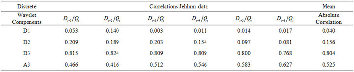
The effectiveness of wavelet components is determined using the correlation between the observed streamflow data and the wavelet coefficients of different decomposition levels. Tables 3(a) and 3(b) show the correlations between each wavelet component time series and original monthly stream flow data. It is observed that the D1 component shows low correlations. The correlation between the wavelet component D2 and D3 of the monthly stream flow and the observed monthly stream flow data show significantly higher correlations compared to the D1 components. Afterward, the significant wavelet components D2, D3 and approximation (A3) component were added to each other to constitute the new series. For the WLSSVM model, the new series is used as inputs to the LSSVM model and LR model. Figure 3 shows the structure of the WLSSVM model. Figures 4 and 5 show the original streamflow data time and their Ds, that is the time series of 2-month mode (D1), 4-month mode (D2), 8-month mode (D3), approximate mode (A3), and the combinations of effective details and approximation components mode (A2 + D2 + D3). Six different combinations of the new series input data (Table 1) is used for forecasting as in the previous application.
A program code including wavelet toolbox was written in MATLAB language for the development of LSSVM and LR models. The forecasting performances of the wavelet-LSSVM (WLSSVM) models, Linear Regression (LR) and wavlet-regression (WR) are presented in Ta-
 (a)
(a)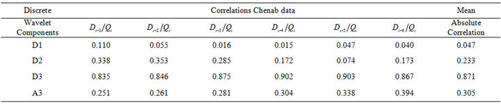 (b)
(b)
Table 3. The correlation coefficients between each of sub-time series and original monthly streamflow data.
Figure 3. The structure of the WLSSVM and WR models.

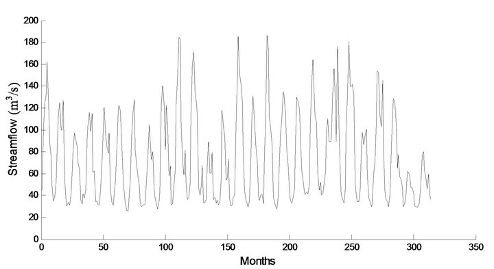
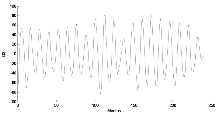
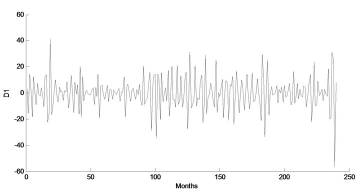
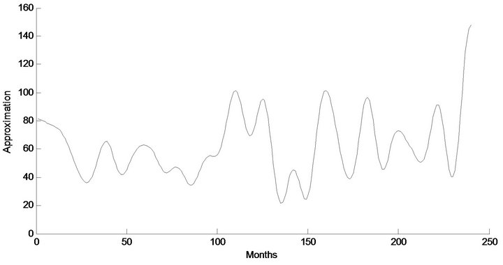
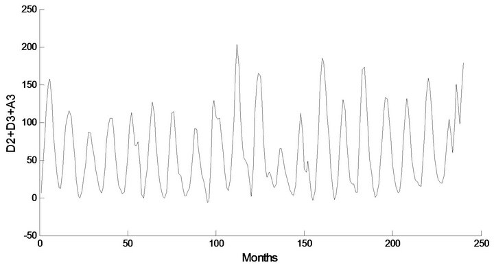
Figure 4. Decomposed wavelet sub-series components (Ds) of streamflow data of Jhelum Station.
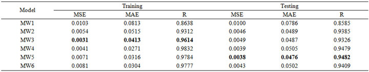
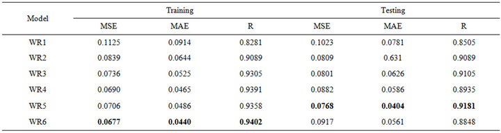
bles 4(a) and 4(b), Tables 5(a) and 5(b) and Tables 6(a) and 6(b) respectively, in terms of MSE, MAE and R in training and testing periods.
Tables 4(a) and 4(b) show that WLSSVM model has a significant positive effect on streamflow forecast. As seen from Table 4(a), for the Jhelum station, the MW3 model has the smallest MSE (0.0031) and MAE (0.0413) and the highest R (0.9614) in the training phase. How-
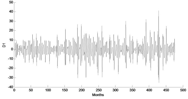
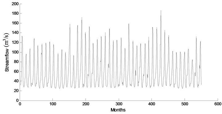
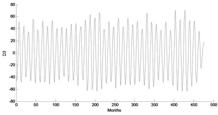
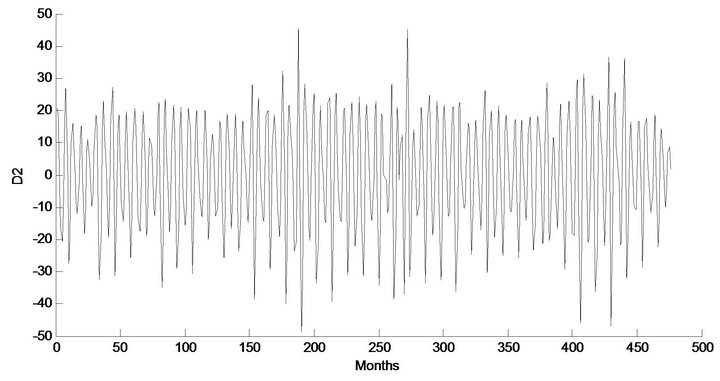
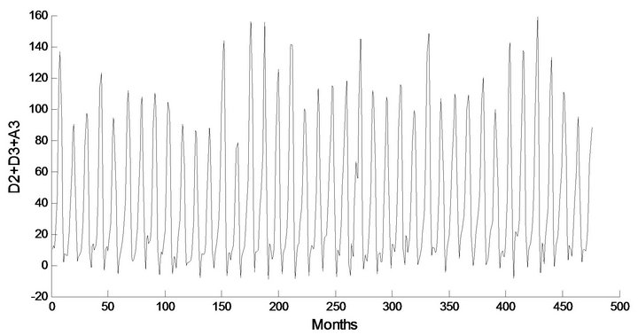

Figure 5. Decomposed wavelet sub-series components (Ds) of streamflow data of Chenab Station.
 (a)
(a)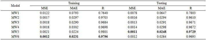 (b)
(b)
Table 4. Forecasting performance indicates of WLSSVM for (a) Jhelum River of Pakistan; (b) Chenab River of Pakistan.
 (a)
(a)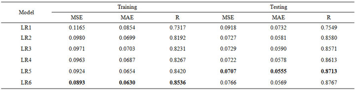 (b)
(b)
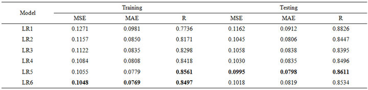
Table 5. Forecasting performances indicates of LR for (a) Jhelum River of Pakistan; (b) Chenab River of Pakistan.
 (a)
(a)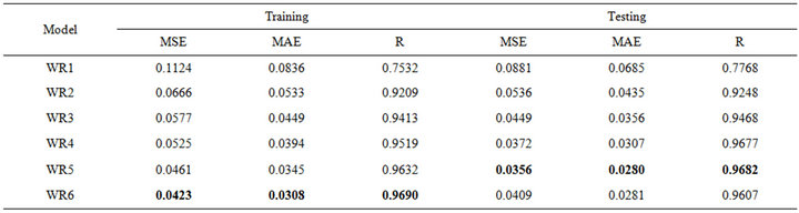 (b)
(b)
Table 6. Forecasting performances indicates of WR for (a) Jhelum River of Pakistan; (b) Chenab River of Pakistan.
ever, for the testing phase, the best MSE (0.0038), MAE (0.0476) and R (0.9482) was obtained for the model input combination MW5. From Tables 5(a) and 5(b) for Chenab station, the MW6 model has the smallest MSE (0.0012) and MAE (0.0231) and the highest R (0.9796) in the training phase. However, for the testing phase, the best MSE (0.0011) and MAE (0.0248) and R (0.9729) was obtained for the model input combination MW5.
5.3. Comparisons of Forecasting Models
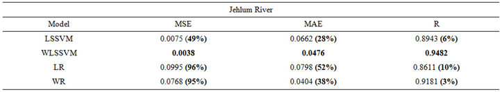
For further analysis, the best performances of the LSSVM, LR, WLSSVM and WR models in terms of the MSE, MAE and R at testing phase are compared.
In Tables 7(a) and 7(b), it shows that WLSSVM has good performance during the testing phase, and they outperform LSSVM, LR and WR in terms of all the standard statistical measures. The correlation coefficient (R) for Jehulm River and Chenab River data obtained by LSSVM models is 0.8943 and 0.9203 and by WR models is 0.9181 and 0.9682 respectively, with WLSSVM model, the R value is increased to 0.9482 and 0.9729. The MSE obtained by LSSVM models is 0.0075 and 0.0035 for both data sets respectively with WLSSVM model this value is decreased to 0.0038 and 0.0011. Similarly, while the MAE obtained by LSSVM is 0.0662 and 0.0430, the MAE value of WLSSVM model is decreased to 0.0476 and 0.0248. The WLSSVM model obtained the best value of MSE and MAE decrease 49% and 69%, respectively, and the best of R increases by 6% compared with single LSSVM model for Jhulem data. For Chenab data the best of R increases by 6% and the best value obtained for MSE and MAE decreases 28% and 42%.
Figures 6 and 7 show the hydrograph and scatter plot for the LSSVM, WLSSVM, WR and LR models for the testing period. It can be seen that the WLSSVM forecasts quite close to the observed data for both station.
The performance of WLSSVM in predicting the streamflow is superior to the classical LSSVM model. As seen from the fit line equations (assume that the equation is ) in the scatterplots that a and b coefficients for the LSSVM, WLSSVM, WR and LR models, respectively, the WLSSVM has less scattered estimates and the R value of WLSSVM model close to 1 (
 and
and ) compared to the LSSVM, WR and LR models for both data sets respectively. Overall, it can be
 (a)
(a) (b)
(b)
Table 7. The performance results LSSVM, WLSSVM, LR and WR approach during testing period.
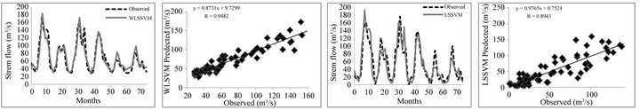
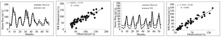
Figure 6. Predicted and observed streamflow during testing period by WLSSVM, LSSVM, LR and WR for Jhelum Station.
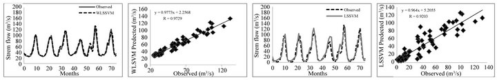
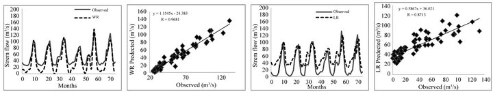
Figure 7. Predicted and observed streamflow during testing period by LSSVM and WLSSVM for Chenab Station.
concluded the WLLSVM model at both studies provided more accurate forecasting results than the LSSVM, WR and LR models for streamflow forecasting.
6. Conclusions
The new method based on the WLSSVM is developed by combining the discrete wavelet transforms (DWT) and least square support vector machines (LSSVM) model for forecasting streamflows. The monthly streamflow time series is decomposed at different decomposition levels by DWT. Each of the decompositions carries most of the information and plays a distinct role in original time series. The correlation coefficients between each of the sub-series and original streamflow series are used for the selection of the LSSVM model inputs and for the determination of the effective wavelet components on streamflow. The monthly streamflow time series data are decomposed at 3 decomposition levels (2 - 4 - 8 months). The sum of effective details and the approximation component were used as inputs to the LSSVM model. The WLSSVM models are trained and tested by applying different input combinations of monthly streamflow data of Chanari station in Jhelum River and Marala station in Chenab in Punjab of Pakistan. Then, LSSVM model is constructed with new series as inputs and original streamflow time series as output. The performance of the proposed WLSSVM model is then compared to the regular LSSVM model for monthly streamflow forecasting.
Comparison results carried out in the study indicated that the WLSSVM model was substantially more accurate than LSSVM, LR and WR models. The study concludes that the forecasting abilities of the LSSVM model are found to be improved when the wavelet transformation technique is adopted for the data pre-processing. The decomposed periodic components obtained from the DWT technique are found to be most effective in yielding accurate forecast when used as inputs in the LSSVM models.
REFERENCES
- H. E. Hurst, “Long Term Storage Capacity of Reservoirs,” Transactions of ASCE, Vol. 116, 1961, pp. 770- 799.
- N. C. Matalas, “Mathematical Assessment of Symmetric Hydrology,” Water Resources Research, Vol. 3, No. 4, 1967, pp. 937-945. doi:10.1029/WR003i004p00937
- G. E. P. Box and G. M. Jenkins, “Time Series Analysis Forecasting and Control,” Holden Day, San Francisco, 1970.
- J. W. Delleur, P. C. Tao and M. L. Kavvas, “An Evaluation of the Practicality and Complexity of Some Rainfall and Runoff Time Series Model,” Water Resources Research, Vol. 12, No. 5, 1976, pp. 953-970. doi:10.1029/WR012i005p00953
- V. Vapnik, “The Nature of Statistical Learning Theory,” Springer Verlag, Berlin, 1995. doi:10.1007/978-1-4757-2440-0
- P. S. Yu, S. T. Chen and I. F. Chang, “Support Vector Regression for Real-Time Flood Stage Forecasting,” Journal of Hydrology, Vol. 328, No. 3-4, 2006, pp. 704-716. doi:10.1016/j.jhydrol.2006.01.021
- Y. B. Dibike, S. Velickov, D. P. Solomatine and M. B. Abbott, “Model Induction with Support Vector Machines: Introduction and Applications,” Journal of Computing in Civil Engineering, Vol. 15, No. 3, 2001, pp. 208-216. doi:10.1061/(ASCE)0887-3801(2001)15:3(208)
- A. Elshorbagy, G. Corzo, S. Srinivasulu and D. P. Solomatine, “Experimental Investigation of the Predictive Capabilities of Data Driven Modeling Techniques in Hydrology, Part 1: Concepts and Methodology,” Hydrology and Earth System Sciences Discussions, Vol. 6, 2009, pp. 7055-7093.
- A. Elshorbagy, G. Corzo, S. Srinivasulu and D. P. Solomatine, “Experimental Investigation of the Predictive Capabilities of Data Driven Modeling Techniques in Hydrology, Part2: Application,” Hydrology and Earth System Sciences Discussions, Vol. 6, 2009, pp. 7095-7142.
- T. Asefa, M. Kemblowski, M. McKee and A. Khalil, “Multi-Time Scale Stream Flow Predictions: The Support Vector Machines Approach,” Journal of Hydrology, Vol. 318, No. 1-4, 2006, pp. 7-16.
- J. Y. Lin, C. T. Cheng and K. W. Chau, “Using Support Vector Machines for Long-Term Discharge Prediction,” Hydrological Sciences Journal, Vol. 51, No. 4, 2006, pp. 599-612. doi:10.1623/hysj.51.4.599
- W. C. Wang, K. W. Chau, C. T. Cheng and L. Qiu, “A Comparison of Performance of Several Artificial Intelligence Methods for Forecasting Monthly Discharge Time Series,” Journal of Hydrology, Vol. 374, No. 3-4, 2009, pp. 294-306. doi:10.1016/j.jhydrol.2009.06.019
- J. A. K. Suykens and J. Vandewalle, “Least Squares Support Vector Machine Classifiers,” Neural Processing Letters, Vol. 9, No. 3, 1999, pp. 293-300. doi:10.1023/A:1018628609742
- D. Hanbay, “An Expert System Based on Least Square Support Vector Machines for Diagnosis of Valvular Heart Disease,” Expert Systems with Applications, Vol. 36, No. 4, 2009, pp. 8368-8374.
- Y. W. Kang, J. Li, C. Y. Guang, H.-Y. Tu, J. Li and J. Yang, “Dynamic Temperature Modeling of an SOFC Using Least Square Support Vector Machines,” Journal of Power Sources, Vol. 179, No. 2, 2008, pp. 683-692. doi:10.1016/j.jpowsour.2008.01.022
- B. Krishna, Y. R. Satyaji Rao and P. C. Nayak, “Time Series Modeling of River Flow Using Wavelet Neutral Networks,” Journal of Water Resources and Protection, Vol. 3, No. 1, 2011, pp. 50-59. doi:10.4236/jwarp.2011.31006
- L. C. Simith, D. L. Turcotte and B. Isacks, “Streamflow Characterization and Feature Detection Using a Discrete Wavelet Transform,” Hydrological Processes, Vol. 12, No. 2, 1998, pp. 233-249. doi:10.1002/(SICI)1099-1085(199802)12:2<233::AID-HYP573>3.0.CO;2-3
- D. Wang and J. Ding, “Wavelet Network Model and Its Application to the Prediction of Hydrology,” Nature and Science, Vol. 1, No. 1, 2003, pp. 67-71.
- D. Labat, R. Ababou and A. Mangin, “Rainfall-Runoff Relations for Karastic Springs: Part II. Continuous Wavelet and Discrete Orthogonal Multiresolution Analysis,” Journal of Hydrology, Vol. 238, No. 3-4, pp. 2000, pp. 149-178. doi:10.1016/S0022-1694(00)00322-X
- S. G. Mallat, “A Theory for Multi Resolution Signal Decomposition: The Wavelet Representation,” IEEE Transactions on Pattern Analysis and Machine Intelligence, Vol. 11, No. 7, 1998, pp. 674-693.
- A. Grossman and J. Morlet, “Decomposition of Harley Functions into Square Integral Wavelets of Constant Shape,” SIAM Journal on Mathematical Analysis, Vol. 15, No. 4, 1984, pp. 723-736. doi:10.1137/0515056
- I. Daubechies, “Orthogonal Bases of Compactly Supported Wavelets,” Communications on Pure and Applied Mathematics, Vol. 41, No. 7, 1988, pp. 909-996. doi:10.1002/cpa.3160410705
- E. Foufoula-Georgiou and P. E Kumar, “Wavelets in Geophysics,” Academic, San Diego and London, 1994.
- R. M. Rao and A. S. Bopardikar, “Wavelet Transforms: Introduction to Theory and Applications,” Addison Wesley Longman, Inc., Reading, 1998, 310 p.
- M. Kucuk and N. Agiralioğlu, “Wavelet Regression Technique for Streamflow Prediction,” Journal of Applied Statistics, Vol. 33, No. 9, 2006, pp. 943-960. doi:10.1080/02664760600744298
- O. Kisi, “Wavelet Regression Model as an Alternative to Neural Networks for Monthly Streamflow Forecasting,” Hydrological Processes, Vol. 23, No. 25, 2009, pp. 3583- 3597. doi:10.1002/hyp.7461
- O. Kisi, “Wavelet Regression Model for Short-Term Streamflow Forecasting,” Journal of Hydrology, Vol. 389, No. 3-4, 2010, pp. 344-353. doi:10.1016/j.jhydrol.2010.06.013
- P. Y. Ma, “A Fresh Engineering Approach for the Forecast of Financial Index Volatility and Hedging Strategies,” PhD thesis, Quebec University, Montreal, 2006.
- M. Firat, “Comparison of Artificial Intelligence Techniques for River Flow Forecasting,” Hydrology and Earth System Sciences, Vol. 12, No. 1, 2008, pp. 123-139.
- R. Samsudin, S. Ismail and A. Shabri, “A Hybrid Model of Self-Organizing Maps (SOM) and Least Square Support Vector Machine (LSSVM) for Time-Series Forecasting,” Expert Systems with Applications, Vol. 38, No. 8, 2011, pp. 10574-10578.
- M. T. Gencoglu and M. Uyar, “Prediction of Flashover Voltage of Insulators Using Least Square Support Vector Machines,” Expert Systems with Applications, Vol. 36, No. 7, 2009, pp. 10789-10798. doi:10.1016/j.eswa.2009.02.021
- L. Liu and W. Wang, “Exchange Rates Forecasting with Least Squares Support Vector Machines,” International Conference on Computer Science and Software Engineering, Wuhan, 12-14 December 2008, pp. 1017-1019.