Open Journal of Statistics
Vol.3 No.2(2013), Article ID:30157,24 pages DOI:10.4236/ojs.2013.32011
Cross-Validation, Shrinkage and Variable Selection in Linear Regression Revisited
1Department of Medical Statistics and Bioinformatics, Leiden University Medical Center, Leiden, The Netherlands
2Institut fuer Medizinische Biometrie und Medizinische Informatik, Universitaetsklinikum Freiburg, Freiburg, Germany
Email: wfs@imbi.uni-freiburg.de
Copyright © 2013 Hans C. van Houwelingen, Willi Sauerbrei. This is an open access article distributed under the Creative Commons Attribution License, which permits unrestricted use, distribution, and reproduction in any medium, provided the original work is properly cited.
Received December 8, 2012; revised January 10, 2013; accepted January 26, 2013
Keywords: Cross-Validation; LASSO; Shrinkage; Simulation Study; Variable Selection
ABSTRACT
In deriving a regression model analysts often have to use variable selection, despite of problems introduced by datadependent model building. Resampling approaches are proposed to handle some of the critical issues. In order to assess and compare several strategies, we will conduct a simulation study with 15 predictors and a complex correlation structure in the linear regression model. Using sample sizes of 100 and 400 and estimates of the residual variance corresponding to R2 of 0.50 and 0.71, we consider 4 scenarios with varying amount of information. We also consider two examples with 24 and 13 predictors, respectively. We will discuss the value of cross-validation, shrinkage and backward elimination (BE) with varying significance level. We will assess whether 2-step approaches using global or parameterwise shrinkage (PWSF) can improve selected models and will compare results to models derived with the LASSO procedure. Beside of MSE we will use model sparsity and further criteria for model assessment. The amount of information in the data has an influence on the selected models and the comparison of the procedures. None of the approaches was best in all scenarios. The performance of backward elimination with a suitably chosen significance level was not worse compared to the LASSO and BE models selected were much sparser, an important advantage for interpretation and transportability. Compared to global shrinkage, PWSF had better performance. Provided that the amount of information is not too small, we conclude that BE followed by PWSF is a suitable approach when variable selection is a key part of data analysis.
1. Introduction
In deriving a suitable regression model analysts are often faced with many predictors which may have an influence on the outcome. We will consider the low-dimensional situation with about 10 to 30 variables, the much more difficult task of analyzing ‘omics’ data with thousands of measured variables will be ignored. Even for 10+ variables selection of a more relevant subset of these variables may have advantages as it results in simpler models which are easier to interpret and which are often more useful in practice. However, variable selection can introduce severe problems such as biases in estimates of regression parameters and corresponding standard errors, instability of selected variables or an overoptimistic estimate of the predictive value [1-4].
To overcome some of theses difficulties several proposals were made during the last decades. To assess the predictive value of regression model cross-validation is often recommended [2]. For models with a main interest in a good predictor the LASSO by [5] has gained some popularity. By minimizing residuals under a constraint it combines variable selection with shrinkage. It can be regarded, in a wider sense, as a generalization of an approach by [2], who propose to improve predictors with respect to the average prediction error by multiplying the estimated effect of each covariate with a constant, an estimated shrinkage factor. As the bias caused by variable selection is usually different for individual covariates, [4] extends their idea by proposing parameterwise shrinkage factors. The latter approach is intended as a post-estimation shrinkage procedure after selection of variables. To estimate shrinkage factors the latter two approaches use cross-validation calibration and can also be used for GLMs and regression models for survival data.
When building regression models it has to be distinguished whether the only interest is a model for prediction or whether an explanatory model, in which it is also important to assess the effect of each individual covariate on the outcome, is required. Whereas the mean square error of prediction (MSE) is the main criterion for the earlier situation, it is important to consider further quality criteria for a selected model in the latter case. At least interpretability, model complexity and practical usefulness are relevant [6]. For the low-dimensional situation we consider backward elimination (BE) as the most suitable variable selection procedure. Advantages compared to other stepwise procedure were given by [7]. For a more general discussion of issue in variable selection and arguments to favor BE to other stepwise procedures and to subset selection procedures using various penalties (e.g. AIC and BIC) see [4] and [8]. To handle the important issue of model complexity we will use different nominal significance levels of BE. The two post-estimation shrinkage approaches mentioned above will be used to correct parameter estimates of models selected by BE. There are many other approaches for model building. Despite of its enormous practical importance hardly any properties are known and the number of informative simulation studies is limited. As a result many issues are hardly understood, guidance to built multivariable regression models is limited and a large variety of approaches is used in practice.
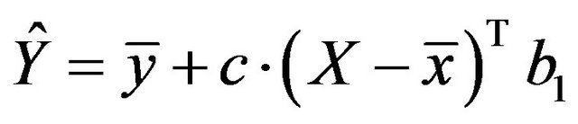
We will focus on a simple regression model
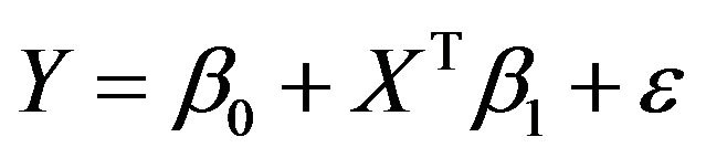
with X a p-dimensional covariate. Let there be n observations  used to obtain estimates
![]() and
and  of the regression parameters.
The standard approach without variable selection is classic ordinary least squares (OLS). In a simulation study we will investigate how much model building can be improved by variable selection and cross-validated based shrinkage. The paper reviews and extends early work by the authors [2,4,9]. Elements added are a thorough reflection on the value of cross-validation and a comparison with Tibshirani’s LASSO [5]. With an interest in deriving explanatory models we will not only use the MSE as criteria, but will also consider model complexity and the effects of individual variables. Two larger studies analyzed several times in the literature will also be used to illustrate some issues and to compare results of the procedures considered.
The paper is structured in the following way. Section 2 describes the design of the simulation study. Section 3 reviews the role of cross-validation in assessing the prediction error of a regression model and studies its behavior in the simulation study. Section 4 reviews global and parameterwise shrinkage and assesses the performance of cross-validation based shrinkage in the simulation data. The next Sections 5 and 6 discuss the effect of model selection by BE and the usefulness of crossvalidation and shrinkage after selection. Section 7 compares the performance of post-selection shrinkage with the LASSO. Two real-life examples are given in Section 8. Finally, the findings of the paper are summarized and discussed in Section 9.
2. Simulation Design
The properties of the different procedures are investigated by simulation using the same design as in [10]. In that design the number of covariates , the covariates have a multivariate normal distribution with mean
 , standard deviation
  for all covariates. Most correlations are zero, except R1,5 = 0.7, R1,10 = 0.5, R2,6 = 0.5, R4,8 = −0.7,
 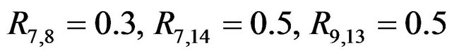 and
and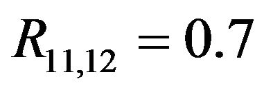 . The covariates
  and
and  are uncorrelated with all other ones. The regression coefficients are taken to be
  (intercept), β1 = β2 = β3 = 0, β4 = −0.5, β5 = β6 = β7 = 0.5, β8 = β9 = 1 and
 ,
, .
.
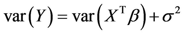
The variance of the linear predictor
 in the model equals
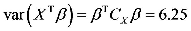 , where CX is the covariance matrix of the X’s. The residual variances are taken to be
  or
or . The corresponding values of the multiple correlation coefficient
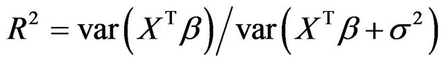 are
are  and
and
 , respectively. Sample sizes are n = 100 or
 . For each of the four
  combinations, called scenarios,
  samples are generated and analyzed. The scenarios are ordered on the amount of information they carry on the regression coeffients. Scenario 1 is the combination
 , scenario 2 is
 , scenario 3 is
 and scenario 4 is
 .
.
Since the covariates are not independent, the contribution of Xj to the variance of the linear predictor
 is not simply equal to
 . Moreover, the regression coefficients have no absolute meaning, but depend on which other covariates are in the model. To demonstrate this, it is studied how dropping one of the covariates influences the optimal regression coefficients of the other covariates, the variance of the linear predictor
  and the increase of the residual variance
 , which is equal to the decrease of
 . This is only done for
  which have non-zero coefficients in the full model. The results are shown in Table 1.
Table 1. Effects of dropping one covariate with non-zero β’s. The other 14 covariates remain in the model. The main body of the table gives the regression coefficients. The last rows show the resulting values of , the increase in the residual variance
  and the multiple correlation R2. The latter is computed for the case of
 . Covariates X1, X2, X3, X11, ..., X15 have β = 0. Dropping them will not affect the β’s of the model under “none”.
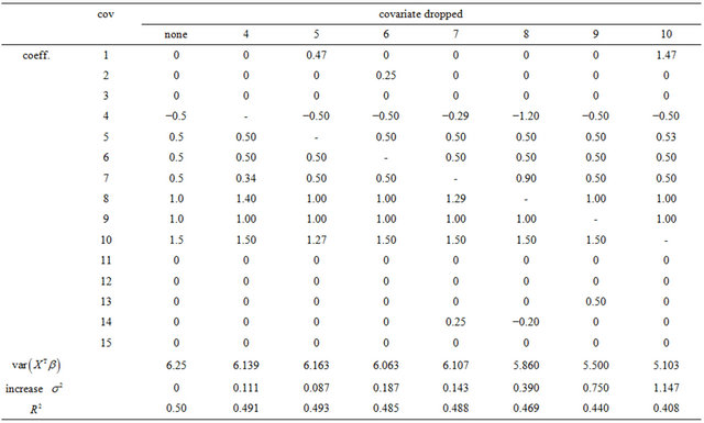
The table also shows the resulting  for the case that
 . Apparently, the effect of each covariate is partly “inherited” by some of the other covariates. A simple pattern of inheritance is seen for X6. It only correlates with X2 and the pair
 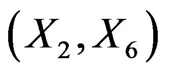 is independent of the rest. If X6 is dropped,
  gets the regression coefficient
 . This saves a little bit of the variance of the linear predictor. It drops from 6.250 to 6.063, while it would have dropped to 6.000 if X6 were independent of the other predictors. A more complicated pattern is seen for X7. If that one is dropped,
  and
and  inherite the effects. The covariates X14 and X8 show up because they are directly correlated with X7. Covariate X4 shows up because it is correlated with X8. The variance of the linear predictor drops from 6.250 to 6.107.
Since  are independent of the other covariates, they cannot inherit effects. However,
  can partly substitute
 , although they have coefficients
  in the full model.
3. The Value of Cross-Validation
Cross-validation is often recommended as a robust way of assessing the predictive value of a statistical model. The simplest approach is leave-one-out cross-validation in which each observation is predicted from a model using all the other observations. The generalization is  -fold cross-validation in which the observations are randomly divided into
  “folds” of approximately equal size and observation in one fold are predicted using the observations in the other folds. In the paper leave-one-out crossvalidation will be used
 , but the formulas presented apply more generally. Let
  be obtained in the cross-validation subset, in which observation
  is not included. The cross-validation based estimate of the prediction error is defined as
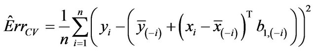
The true prediction error of the model with estimates b0 and b1 from the “original” model using all n observations is defined as
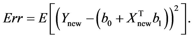
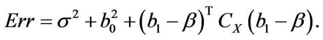
In the simulation study it is given by
The results in the simulation study using all covariates without any selection are given in Table 2.
The results show that  does a good job in estimating the mean value of
  over all simulations. However, since the correlation between
  and
and  over all simulation runs is virtually equal to zero, it must be concluded that it does a very poor job in estimating the prediction error of the individual models.
Notice that the standard deviation of  is much larger than that of
 . The explanation is that a lot of the variation in
  is due to the estimation of the unknown
 . Cross-validation might be do a better job in picking up the systematic prediction part of the prediction error caused by the error in the estimated
 ’s. That can be checked by studying the behavior of
 which is an estimate of the systematic part
 . Here
  is the usual unbiased estimator of
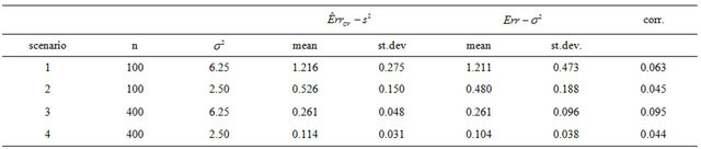
 . The results are shown in Table 3. It nicely shows that the systematic error decreases monotonically from scenario 1 to scenario 4.
Means are very similar but standard deviations from the CV estimates are much smaller. CV somehow shrinks the estimate of the systematic error towards the mean. The table shows that the correlations between the estimate  and the true value
  are still very low. The warning issued in Section 4 of [2] still holds. It is nearly impossible to estimate the prediction error of a particular regression model. Cross-validation is of very little help in estimating the actual error. It can only estimate the mean error, averaged over all potential
“training sets”. However, it might be helpful in selecting procedures that reduce the prediction error.
Finally, it should be pointed out that the cross-validation results are in close agreement with the model based estimates of the prediction error as discussed in the same section of [2].
4. Cross-Validation Based Shrinkage without Selection
4.1. Global Shrinkage
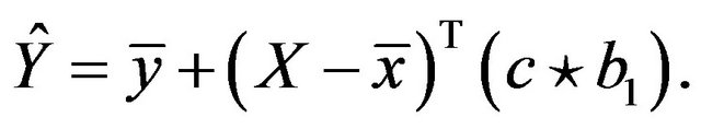
As argued by [2,11], the predictive performance of the resulting model can be improved by shrinkage of the model towards the mean. This gives the predictor
with shrinkage factor c, . In the following c will be called global shrinkage factor. Under the assumption of homo-skedasticity, the optimal value for c can be estimated as
with  the explained sum of squares,
  the estimate of the residual variance and p the number of predictors.
A model free estimator can be obtained by means of cross-validation. Let  be obtained in the cross-validation subset, in which observation
  is not included, then
 ![]() can be estimated by minimizing
can be estimated by minimizing
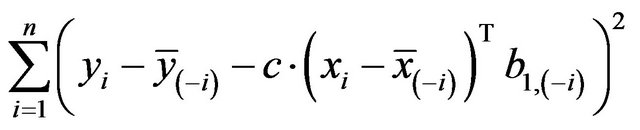
Table 2. Simulation results for  and
and  and their correlation (corr.) in models without selection.
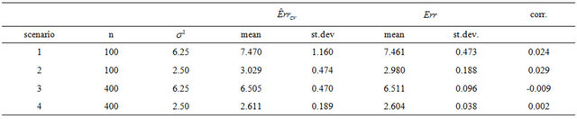
Table 3. Simulation results for  and
and  and their correlation (corr.) in models without selection.
resulting in
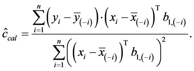
This estimate can be obtained by regressing 
on  in a model without an intercept. It differs slightly from the one obtained by regressing
  on
on ![]() as proposed in [2]. The definition allows k-fold cross-validation and is not restricted to leave-one-out cross-validation. The results of application of global shrinkage in the simulation data, ignoring the restriction
as proposed in [2]. The definition allows k-fold cross-validation and is not restricted to leave-one-out cross-validation. The results of application of global shrinkage in the simulation data, ignoring the restriction , are shown in Table 4. Actually,
  was never observed and
  only occasionally.
The table shows that global shrinkage can help to reduce the prediction error if the amount of information in the data is low. For scenario 1 the mean of the shrinkage factor is 0.84 and the mean reduction of prediction error is 0.14. Corresponding values for scenario 4 are 0.98 and 0.001. For the latter all shrinkage factors are close to one and predictors with and without shrinkage are nearly identical. However, the positive correlation between the shrinkage factor c and the reduction in prediction error is counter-intuitive. To get more insight the data for scenario 1 with a small amount of information  is shown in Figure 1.
The relation between reduction in prediction error due to shrinkage and the prediction error of the OLS models are shown for three categories of the shrinkage factor c, namely  and
and . The frequencies of these categories among the 10,000 simulations are 1754, 7740 and 506, respectively. The upper panel shows the apparent (estimated) prediction errors based on cross-validation and the apparent reduction achieved by global shrinkage. The differences between the three categories are small, but they are in line with the intuition that the largest reduction is achieved when the shrinkage factor is small. The quartiles (25%, 50%, 75%) of the apparent reduction are 0.09, 0.15, 0.27 for
  for
for  and −0.07−0.02, 010 for
 . The middle panel shows the actual (true) prediction error based on our knowledge of the true model. Here, the picture is completely different. Reduction of the prediction error only occurs when the shrinkage factor is close to one and the OLS prediction error is large. Substantial shrinkage with
  tends to increase the prediction error. The quartiles of the true reduction are −0.29, −0.13, 0.04 for c < 0.8, 0.05, 0.18, 0.31 for
  and 0.19, 0.28, 0.38 for
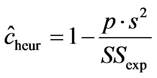
 . The lower panel shows the relation between the apparent and the actual reduction. At first sight the results our counter-intuitive. This phenomenon is extensively discussed in [9]. What happens could be understood from the heuristic shrinkage factor
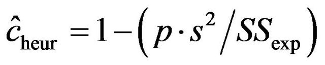 . If
. If  is “large” by random fluctuation, the observed explained sum of squares
  is large and
  stays close to 1 and does not “push”
  in the direction of the true
 . If
. If  is “small” by random fluctuation,
  is small and
  will be closer to 0 and might “push” in the wrong direction. This explains the overall negative correlation
  between apparent and actual reduction of the prediction error. It must be concluded that it is impossible to predict from the data whether shrinkage will be helpful for a particular data set or not. The chances are given under “frac. pos.” in Table 4. They are quite high in noisy data, but that gives no guarantee for a particular data set.
4.2. Parameterwise Shrinkage
[4] suggested a covariate specific shrinkage factor, coined parameterwise shrinkage factor (PWSF), to be defined as
Here, ![]() is a vector of shrinkage factors with
is a vector of shrinkage factors with  for
for  and “
and “ ” stands for coordinate-wise multiplication:
 . This way of regulation is in the spirit of Breiman’s Garrote [12]. See also [9,13]. Sauerbrei suggests to use the parameterwise shrinkage after model selection and to estimate the vector
 ![]() by cross-validation. As for the global shrinkage
by cross-validation. As for the global shrinkage
Table 4. Simulation results for the reduction in prediction error (compared with OLS) achieved by global shrinkage in models without selection; “frac. pos.” stands for the fraction with positive reduction, “corr.” stand for the correlation between the shrinkage factor and the reduction.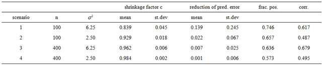
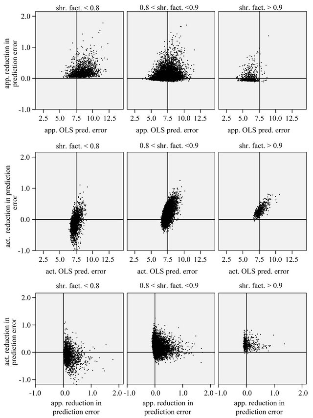
Figure 1. Reduction of prediction error achieved by global shrinkage for different categories of the shrinkage factor c; data from scenario 1 . The upper panel shows the apparent prediction errors obtained through crossvalidation, the middle panel shows the actual (true) prediction errors and the lower panel shows the relation between the apparent and the actual reduction.
this could be obtained by regression without intercept of  on
on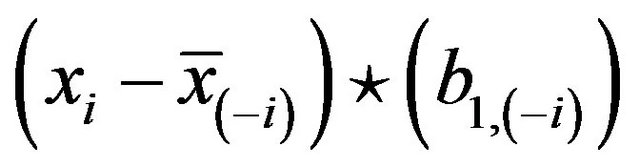 .
.
Although this is against the advice of [4] parameterwise shrinkage was applied in the simulation data in models without selection, ignoring the restrictions  for
for . A summary of the results is given in Table 5.
Using PWSF the average prediction error increases when compared with the OLS predictor. The increase is large (about 10%) in scenario 1. In scenario 4 the increase is moderate, but still present. Moreover, the estimated prediction error obtained from the cross-validation fit is far too optimistic. (Data not shown). The explanation is that parameterwise shrinkage is not able to handle the redundant covariates with no effect at all. This can be seen from the box plots in Figure 2.
For the redundant covariates the shrinkage factors are all over the place. Even variables with a weak effect have sometimes negative PWSF values. For the strong covariates they are quiet well-behaved despite the erratic behavior for the other ones. The conclusion must be that
Table 5. Comparison of the prediction errors of OLS, global shrinkage and parameterwise shrinkage in models without selection.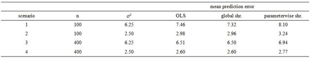
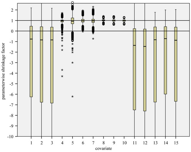
Figure 2. Box plot of parameterwise shrinkage factors in models without selection. Results from scenario 4.
in models with many predictors without selection on stronger predictors parameterwise shrinkage cannot be recommended. The behavior is a bit better if negative shrinkage values will be set to zero, but altogether such a constraint is not sufficient. This is completely in line with Sauerbrei’s original suggestion.
5. Model Selection
Following [10] models are selected by backward elimination at significance levels of  and
and . An impression of which covariates are selected is, shown in Figure 3.
5.1. Number of Variables Selected, Type I and Type II Error
The “softest” definition of model selection is the selection of covariates to be used in further research. The “optimal” model contains only the important covariates, the ones that have an influence on the outcome in the full model. In the simulation those are the covariates . If these are selected the other ones are redundant. However if one of the important covariates is not selected, other non-important covariates can come to the rescue if they are correlated with the non-selected important covariate(s). In the simulation data non-important covariates that can play such a role are covariates
  as can be seen from Table 1. The effect of omitting important covariates is the loss of explained variation in the optimal model after selection or, equivalently, the introduction of additional random error. If no selection takes place there is no loss of explained variation, but there is a large number of non-important covariates, leading to larger estimation errors. Even more important is a severe loss in general usability of such predictors [4,6]. Consider, for example, a prognostic model comprising many variables. All constituent variables would have to be measured in an identical or at least in a
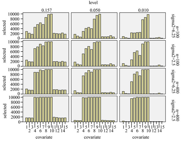
Figure 3. Frequency of selection per covariate.
similar way, even when their effects were very small. Such a model is impractical, therefore “not clinically useful” and likely to be “quickly forgotten” [14].
From Figure 3 we learn that in the easy situation with a lot of information (scenario 4) all important variables are selected in nearly all replications. For the 8 variables without an influence selection frequencies agree closely to the nominal significance level. For  selection frequencies are between 15.7% and 19.0%. The corresponding relative frequencies are between 5.1% and 6.55% for
  and between 0.9% and 3.3% for
 . Results are much worse for situations with less information. For the most extreme scenario 1 it is obvious that all selected models deviate substantially from the true model. For
  selection frequencies are only between 23.4% and 25.1% for the 4 relevant variables
  with a weak effect. Even for
  these frequencies are only between 46.1% and 57.3%. Of these
  has the lowest frequency, which is probably caused by the strong correlation with
 . With 28.9%
  has the largest frequency of selection among the non-important covariates. That is explained by its strong correlation with X5. In 19.4% of the simulations X1 is selected while the important variable X5 is not selected.
The effect of selection at the three levels is shown in Figures 4-6.
Figure 4 summarizes the number of included variables for the different scenarios. In the simple scenario 4 all seven relevant variables were nearly always selected. In addition irrelevant variables were selected in close agreement to the significance level. In  the correct model was selected for
  whereas redundant variables without influence were added when using
  For scenarios with less information the number of selected variables is usually smaller and the significance level has a stronger influence on the inclusion frequencies. Strong predictors are still selected in most of the replications, but the rest of the selected model does hardly ever agree to the true model. For each of the variables with a weaker effect the power for variable inclusion is low.
The comparison of Figures 5 and 6 nicely shows the balance between allowing redundant covariates (covariates without effect in the selected model) and allowing loss of explained variation. The number of redundant covariates shown in Figure 5, corresponds directly to the type I error. It hardly depends on the residual variance  and the sample size
![]() . Despite of some stronger correlations in our design the distribution is very close to binomial
. Despite of some stronger correlations in our design the distribution is very close to binomial . The type II error is reflected by the loss of the variance of the optimal linear predictor
  , or ,equivalently, the increase in residual variance
 , caused by not selecting all important covariates. It could be translated into a loss of
  by dividing it by the marginal variance
 , which is equal to 12.5 in scenarios 1 and 3 (σ2 = 6.25) and 8.75 in scenarios 2 and 4 (σ2 = 2.5). This is shown in Figure 6.
Generally speaking, loss of  depends on both the significance level used in the selection process and the
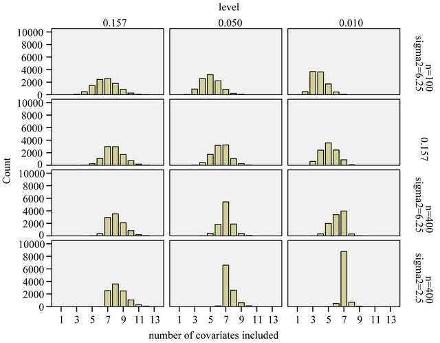
Figure 4. Number of included covariates.
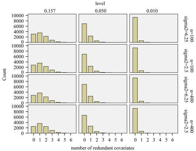
Figure 5. Number of redundant covariates.
amount of information in the data reflected by residual variance  and the sample size
![]() . In scenario 4 with a high amount of information, the loss of
. In scenario 4 with a high amount of information, the loss of  is negligible and the number of redundant covariates can be controlled by taking
 . In scenario 1 there is a substantial loss of
  if the selection is too strict and
  might be more appropriate.
As mentioned above and seen in Table 1 the variable  can partly take over the role of
  (correlation coefficient is 0.7) if the latter is not selected. That is shown in Table 6 for scenario 2 and
 . It has to be kept in mind that other variables are also deleted making a direct comparison difficult. Concerning these two variables the correct model includes X5 and excludes X1, which is the case in 69% of the replications. Here the mean loss is smallest. X5 is erroneously excluded in about 28% of the models. In about half of them the correlated variable X1 is included, reducing the R2 loss
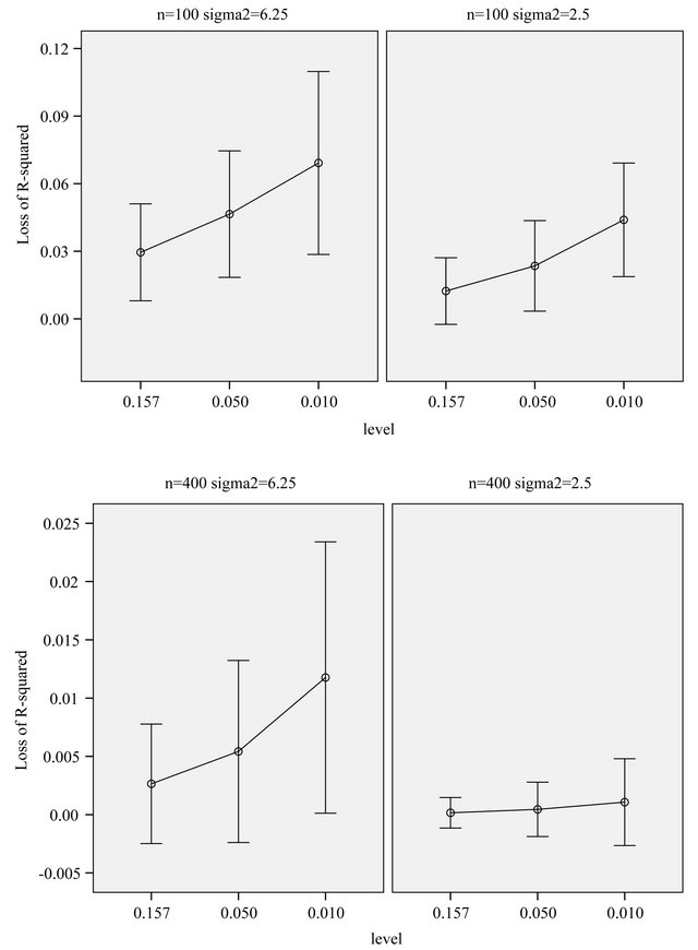
Figure 6. Loss of R2 in comparison to the full model. The bars show mean ± 1 st.dev. in the population of replications.
Table 6. Inclusion frequencies and average loss of  for combinations of
  and
and  for scenario 2 and
 .
.
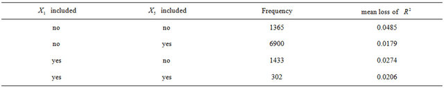
caused by exclusion of X5 substantially.
5.2. Assessment of Prediction Error
The prediction error of a particular model depends on the number of redundant covariates and the loss of explained variation. The average reduction of prediction error when compared with no selection (significance level ) is shown in Figure 7. Those numbers could be best compared with the systematic component of the prediction error,
  , as reported in Table 3.
It nicely shows that the optimal level depends on the amount of information in the data. It also shows that moderate selection at , in a univariate situation equivalent with AIC or Mallows’ CP, can do very little harm. Even
 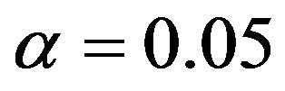 gives always better results than no selection. For a small sample size the relative reduction in prediction error is small. For the large sample size elimination of several variables reduces the relative prediction error substantially for
 . The average number of selected variables is 7.02 for scenario 3 and 7.40 for scenario 4.
Figure 8 shows the prediction error ranking of the different levels in the individual simulation data sets. Mean ranks were used in replications where the same model was selected. As observed before, the variation is very big and there is no outspoken winner, but there are some outspoken losers. In all scenarios it is bad not to select at all. However, for a small sample size it is even worse to use a very small selection level.
The prediction errors of the selected models can be estimated by cross-validation in such a way that in each cross-validation data set the whole selection procedure is carried out. As in Section 3 this will yield a correct estimate of the average prediction. Thus, it could be used to select the “optimal” significance level in general, but it will not necessarily yield the best procedure for the actual data set at hand.
6. Post-Selection Cross-Validation
A common error in model selection is to use crossvalidation after selection to estimate the prediction error and to select the best procedure. As pointed out by [15], this is a bad thing to do. That is exemplified by Figures 9 and 10.
Comparing Figures 7 and 9 shows that cross-validation after selection is far too optimistic about the reduction of the prediction error and is not able to notice the poor performance of selection at  for the scenarios 1 and 2. Moreover, as can be seen from Figure 10, post-selection cross-validation tends to favor selection at
  for all scenarios. This is no surprise because in univariate selection
  is equivalent with using AIC, which is very close to using cross-validated prediction error if the normal model holds true.
6.1. Post-Selection Shrinkage
While cross-validation after selection is not able to select
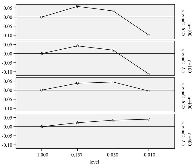
Figure 7. Mean reduction of the true prediction error as reported in Tables 2 and 3 for different α-levels. Values of Err − s2 are 1.21, 0.48, 0.26 and 0.104 in scenarios 1-4, respectively (see Table 3).
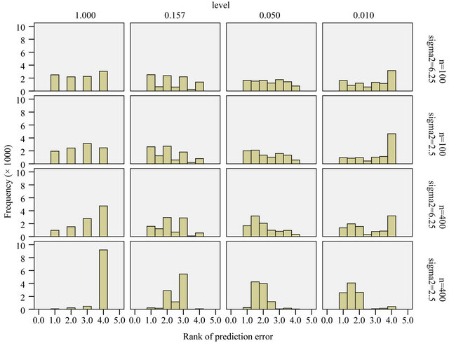
Figure 8. Ranks of prediction error for different levels; rank = 1 is best, rank = 4 is worst.
Figure 9. Reduction of estimated prediction error, obtained through post-selection cross-validation, after backward elimination with three selection levels.
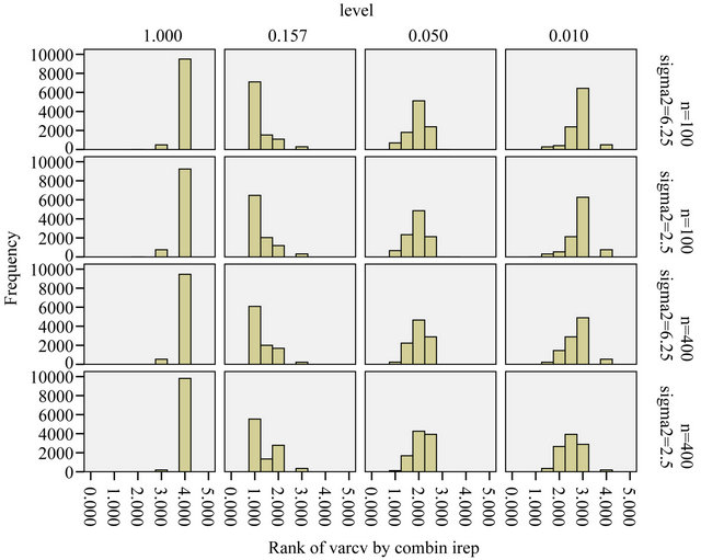
Figure 10. Ranks of estimated prediction error obtained from post-selection cross-validation for different levels; rank = 1 is best, rank = 4 is worst. The ranks of the true prediction error are shown in Figure 8.
the best model, it might be of interest to see whether cross-validation based shrinkage after selection can help to improve the model. The results are shown in Figure 11.
On the average, parameterwise shrinkage gives better predictions than global shrinkage, when applied after selection. An intuitive explanation is that small effects that just survive the selection, are more prone to selection bias and, therefore, can profit from shrinkage. In contrast, selection bias plays no role for large effects and shrinkage is not needed, see [16] and chapter 2 of [8]. Whereas global shrinkage “averages” over all effects, parameterwise shrinkage aims to shrink according to these individual needs.
This can also be investigated by looking into the mean squared estimation errors  of the regression coefficients conditional on the selection of covariates in the model. The coefficients
  are the optimal regression coefficients in the selected model. As discussed in Section 2 the
  coefficients can differ from the
  coefficients if there is correlation between the covariates. Figure 12 shows the mean squared errors of the shrinkage based estimators relative to the mean squared errors of the OLS estimators for sample size
 , scenarios 1 and 2 . Sample size
  is not shown, because post-selection shrinkage has hardly any effect.
It is clear that the parameterwise shrinkage helps to reduce the effect of redundant covariates that only enter by chance, while the global shrinkage is not able to make that distinction. The precise mechanism is not quite clear yet. To get some better feeling what is going on, the observed scatterplot of parameterwise shrinkage factors versus the OLS estimator are shown in Figure 13 for covariate X3 (no effect), X6 (weak effect) and X9 (strong effect). These covariates are selected because the optimal parameter value when selected does not depend on which other covariates are selected as well. X3 is independent of all other variables and the other two variables are only correlated with one variable without influence. Therefore parameter estimates are theoretically equal to the true value in the full model. If the optimal value varies with the selection the graphs are a bit harder to interpret.
For X3, the covariate without effect and no correlation, the inclusion frequency is close to the type I error and in about half of these cases parameter estimates are positive and negative. The variable is selected in replications in which the estimated regression coefficient is by chance most heavily overestimated (in absolute terms) compared to the true (null) effect. One would hope that PWFS would correct these chance inclusions by a rule like “the larger the absolute effect , the smaller the shrinkage factor
![]() ”. Although most shrinkage factors are much lower than one, Figure 13 shows a different cloud: “the larger
”. Although most shrinkage factors are much lower than one, Figure 13 shows a different cloud: “the larger , the larger
![]() ”.
”.
A similar observation transfers to the plot for X9, which is selected in all replications. Therefore, selection bias is no issue for this covariate. The hope is that PWSF would move the estimate close to the true value β = 1.0.
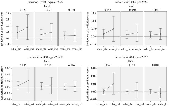
Figure 11. Reduction in prediction error obtained through shrinkage after selection. Error bars show mean ± 1 standard deviation.
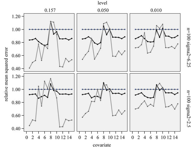
Figure 12. Relative mean squared estimation errors of the partial regression coefficient per covariate (compared to OLS in the selected model) for the parameter estimates obtained by global (black) or parameterwise post-selection shrinkage (grey). Covariates 1-3 and 11-15 have no effect in the full model.
Generally speaking that does not happen: c increases slowly with b. Most values are close to 1, indicating that shrinkage is not required. The only “hoped for” observation can be made for the cases where the correlated
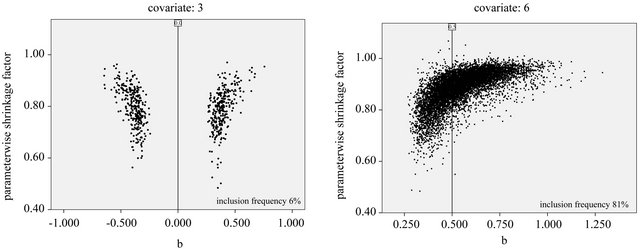
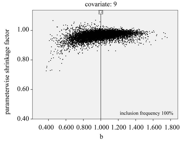
Figure 13. Parameterwise shrinkage factors versus OLS estimates from selected models for covariates 3, 6 and 9; α = 0:05 and scenario 2; reference lines refer to the true value of the parameter.
variable X13 is included (plot not shown). X13 has no effect and the selection frequency (5.9%) agrees well to the type I error. If X13 is included, the shrinkage factor for X9 show a decreasing trend with ![]() -values clearly below 1 if the estimate
-values clearly below 1 if the estimate  overestimates the true value
 , and values around
  if
if . One might say that parameter shrinkages helps to correct for chance inclusions of X13 but not for estimation errors.
X6 is a covariate with a weak effect. It is not included in 19% of the replications, certainly cases in which the true effect was underestimated by chance. The overall picture for the case where it is included shows a stronger increasing trend (compared with X9) tending to a value of about , if b is large. Here, X2 plays the role of a confounding redundant covariate. In cases where it is included (plot not shown), the shrinkage factor for X6 is rather stable with median value about
 .
.
Some understanding can be obtained by the observation in [2] that in univariate models the optimal shrinkage factor is given by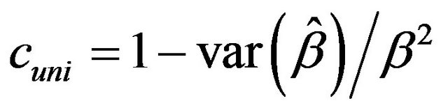 . If
. If  is smallthis quantity is very hard to estimate. If
  is large it could be estimated by
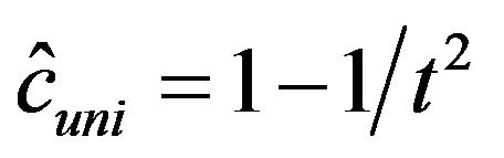 . The parameterwise shrinkage factor behaves very similarly. This could be seen from plotting PWSF against
 ![]() (Graphs not shown). Such a plot clearly shows that
(Graphs not shown). Such a plot clearly shows that  (for
(for ) is the cut-point for an inclusion and that PWSF tends to increase with
 ![]() for included variables. For large absolute t-values, PWSF’s are close to one. whereas they drop to about 0.8 for
for included variables. For large absolute t-values, PWSF’s are close to one. whereas they drop to about 0.8 for ![]() close to 2. The relation between PWSF and
close to 2. The relation between PWSF and ![]() is similar for all three covariates
is similar for all three covariates . The difference between the covariates is the size of the effect and correspondingly the range of
 ![]() after selection.
after selection.
The conclusion so far is that coordinate-wise shrinkage is helpful after selection. However it is not clear how to select the significance level. In a real analysis, the level should be determined subjectively by the aim of the study [4]. In the following we will compare backwards elimination with a procedure like the LASSO, that combines selection, shrinkage and fine-tuning.
7. Comparison with LASSO
The simulations discussed above were compared with the results of the LASSO with cross-validation based selection of the penalty parameter![]() . Because LASSO is quite time-consuming it was only applied on the first 2000 data sets for each combination of
. Because LASSO is quite time-consuming it was only applied on the first 2000 data sets for each combination of ![]() and
and . Figure 14 shows the distribution of the cross-validation based
 ![]() for each combination. The variation in the penalty parameter
for each combination. The variation in the penalty parameter![]() , even in the simple situation of scenario 4 is surprisingly large. There is some correlation with the estimated variance in the full model, but that does not explain the huge variation.
, even in the simple situation of scenario 4 is surprisingly large. There is some correlation with the estimated variance in the full model, but that does not explain the huge variation.
The next Figure 15 shows the inclusion frequencies
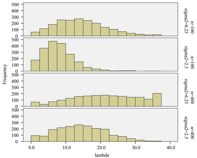
Figure 14. LASSO: histogram of the cross-validation based λ’s for the different scenarios.

Figure 15. LASSO: inclusion frequencies of the covariates.
for the different covariates. Relevant variables are nearly always included, but LASSO is not able to exclude redundant covariates if there is much signal in the other ones. For example, in scenario 4 inclusion frequencies are 52% for  and 54% for
 , the two uncorrelated variables without influence. The probable reason is that selection and shrinkage are controlled by the same penalty term
![]() . The phenomenon is also nicely illustrated by Figure 16.
. The phenomenon is also nicely illustrated by Figure 16.
Finally, the question how the prediction error of LASSO compares with the models based on selection and shrinkage is answered by Figure 17.
The conclusion must be that LASSO is no panacea. Concerning prediction error, it seems to be OK for noisy data (scenarios 1 and 2), but it is beaten by variable selection followed by some form of shrinkage if the data are less noisy (scenario 4). Most likely, that is caused by the inclusion of two many variables without effect. Variable selection combined with parameterwise shrinkage performs quit well. The choice of a suitable significance level seems to depend on the amount of information in the data. Whereas  has the best performance in scenario 4, this level seems to be too low in the other scenarios. In these cases selections with
  or
or  have better prediction performance. Using post selection shrinkage slightly reduces the prediction errors with an advantage for parameterwise shrinkage.
8. Examples
8.1. Ozone Data
For illustration, we consider one specific aspect of a study on ozone effects on school children’s lung growth. The study was carried out from February 1996 to October 1999 in Germany on 1101 school children in first and second primary school classes (6 - 8 years). For more details see [17]. As in [18] we use a subpopulation of 496 children and 24 variables. None of the continuous variables exhibited a strong non-linear effect, allowing to assume a linear effect for continuous variables in our analyses.
First, the whole data set is analyzed using backward elimination in combination with global and parameterwise shrinkage and LASSO. Selected variables with corresponding parameter estimates are given in Table 7 and mean squared prediction errors are shown in Table 8. The t-values are only given for the full model to illustrate the relation between the t-value and the parameterwise shrinkage factor. For variables with very large ![]() -values, PWSF are close to 1. In contrast, PWSFs are all over the place if
-values, PWSF are close to 1. In contrast, PWSFs are all over the place if ![]() is small, a good indication that variables should be eliminated.
is small, a good indication that variables should be eliminated.
Mean squared prediction errors for the full model and the BE models were obtained through double cross-validation in the sense that for each cross-validated prediction, the shrinkage factors were determined by crossvalidation within the cross-validation training set. Prediction error for the LASSO is based on single crossvalidation because double cross-validation turned out to be too time-consuming. Therefore, the LASSO prediction error might be too optimistic.
MSE is very similar for all models, irrespective of applying shrinkage or not (range 0.449 - 0.475; the full model with PWSF is the only exception), but the number
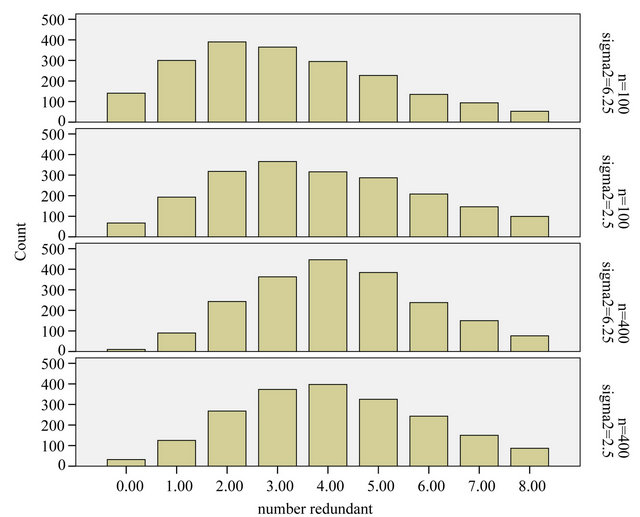
Figure 16. LASSO: distribution of the number of redundant covariates. There are eight redundant covariates in the design.
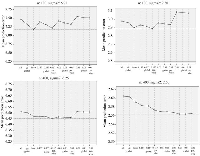
Figure 17. Average prediction errors for different strategies.
Table 7. Analysis of full ozone data set using standardized covariates. The unadjusted R2 equals 0.67 in the full model and drops only slightly to 0.64 for the BE(0.01) model. For the LASSO model it is 0.66.
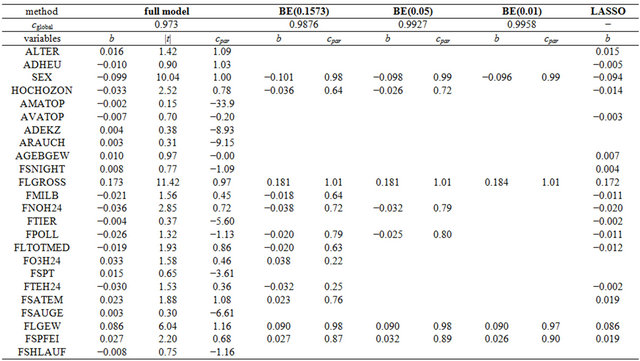
Table 8. Mean squared prediction errors.
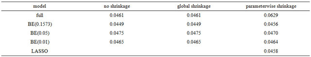
of variables in the model is very different. BE(0.01) selects a model with 4 variables, corresponding PWSF are all close to 1. Three variables are added if 0.05 is used as significance level. Using 0.157 selects a model with 12 variables. Two of them have a very low (below 0.3) PWSF, indicating that these variables may better be excluded. LASSO selects a complex model with 17 variables.
Although they carry relevant information the double cross-validation results for the full data set lack the intuitive appeal of the split-sample approach. To get closer to that intuition the following “dynamic” analysis scheme is applied. First the data are sorted randomly, next the first ![]() observations are used to derive a prediction model which is used to predict the remaining
observations are used to derive a prediction model which is used to predict the remaining  observations. This is done for ntrain = 100, 150, 200, 250, 300, 350 and repeated 100 times. In that way an impression is obtained how the different approaches behave with growing information. The results are shown in graphs. Figure 18 shows the mean number of covariates included. More variables are included with increasing sample size (larger power) and differences between the procedures are substantial. For ntrain = 350 LASSO selects on average 14.4 variables, whereas BE(0.01) selects only 4.0 variables. Figure 19 shows the evolution of the global shrinkage factor. For models selected with BE(0.01) it is always around 0.98 and for BE(0.157) it varies between 0.96 and 0.98, but for the full model the global shrinkage factor is much lower, starting from 0.83 with an increase to 0.95. Figure 20 shows the mean squared prediction errors for the different strategies. Without selection PWSF has a very bad performance, whereas the global shrinkage factor can slightly reduce MSE of prediction. PWSF improves the predictor if variable selection is performed and has smaller MSE than using a global shrinkage factor. The most important conclusion is that “BE(0.01) followed by PWSF” and LASSO have very similar prediction MSE’s, but the LASSO has to include many more covariates to achieve that.
8.2. Body Fat Data
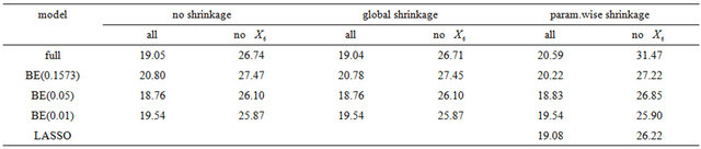
In a second example we will illustrate some issues in a study with one dominating variable. The data were first analysed in [19] and later used in many papers. 13 continuous covariates (age, weight, height and 10 body circumference measurements) are available as predictors for percentage of body fat. As in the book of [8] we excluded case 39 from the analysis. The data are available on the website of the book. In Table 9 we give mean squared prediction errors for several models and shrinkage approaches. Furthermore we give these estimates for variables excluding , the dominating predictor. This analysis assumes that
  would not have been measured or that it would not have been publicly available. A related analysis is presented in chapter 2.7 of [8] with the aim to illustrate the influence of a dominating predictor and to raise the issue about the term “full model” and whether a full model approach has advantageous properties compared with variable selection procedures. Using all variable MSEs of the models are very similar with a range from 18.76 - 20.80. Excluding
  leads to a severe increase, but differences between models are still negligible (25.87 - 27.47); with the full model followed by PWSF as an exception. This agrees well with the results of the ozone data. For BE(0.157), BE(0.01) and LASSO we give parameter estimates in Table 10.
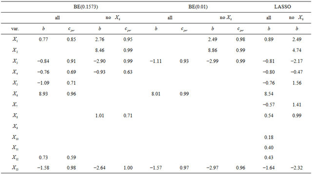
Excluding  results in the inclusion of other variables for all approaches. As in the ozone data LASSO hardly eliminates any variable, but the MSE is not better than from BE(0.01) followed by PWSF. PWSF of all variables selected by BE(0.01) are close to 1, whereas variables selected additionally by BE(0.157) all have PWSF values below 0.9 and sometimes around 0.6. This example confirms that BE(0.01) followed by PWSF gives similar prediction MSE’s, but includes a much smaller number of variables.
9. Discussion and Conclusions
Building a suitable regression model is a challenging task if a larger number of candidate predictors is available. Having a situation with about 10 to 30 variables in mind the full model is often unsuitable and some type of variable selection is required. Obviously subject matter knowledge has to play a key role in model building, but often it is limited [20] and data-driven model-building is required. Despite of some critique in the literature [3,20,
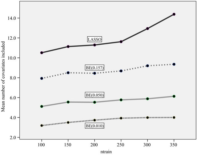
Figure 18. Mean number of covariates included under different strategies.
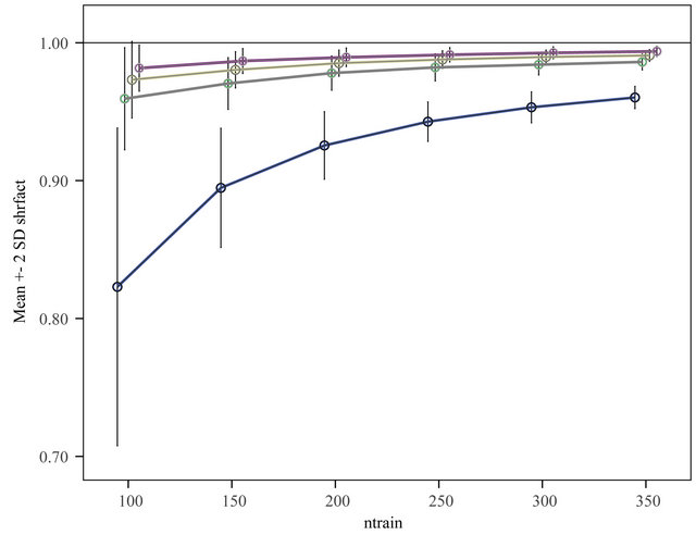
Figure 19. Evolution of the global shrinkage factor for different selection levels. From top to bottom BE(0.010), BE(0.050), BE(0.157) and BE(1.000) = “No selection”.
21] we consider backward elimination as a suitable approach, provided the sample size is not too small and the significance level is sensibly chosen according to the aim of a study. For a more detailed discussion see chapter 2 of [8]. Underand overfitting, model instability and bias of parameter estimates are well known issues of selected regression models.
In a simulation study and two examples we discuss the value of cross-validation, assess a global and a parameterwise cross-validation shrinkage approach, both without and with variable selection, and compare results with the LASSO procedure which combines variable
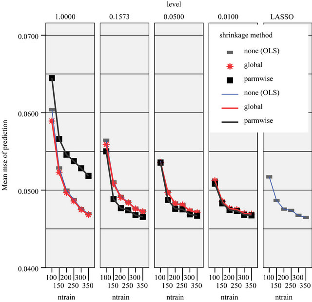
Figure 20. Mean squared prediction error for the different strategies.
Table 9. Mean squared prediction errors.
selection with shrinkage [2,4,5]. As discussed in the introduction it is often necessary to derive a suitable explanatory model which means that the effects of individual variables are important. In this respect a sparse model has advantages, both from a statistical point of view and from a clinical point of view. In a related context [22] refer to parameter sparsity and practical sparsity.
9.1. Design of Simulation Study
Our simulation design was used before for investigations of different issues [10]. We consider 15 covariates with seven of them having an effect on the outcome. In addition, multicollinearity between variables introduces indirect effects of irrelevant variables if a relevant variable is not included. It seems consensus that stepwise and other variable selection procedures have limited value as tools for model building in small studies ([8,21] Section 2.3) and 10 observations per variable is often considered as a lower boundary to derive an explanatory model [23]. Based on this knowledge it is obvious that a sample size of  (6.7 per variable) is low. As a more realistic scenario we also consider
 . Concerning the residual variance we have chosen two scenarios resulting in
  and
and . The 4 scenarios reflect the situation with a low to a large(r) amount of information in the data. As expected from related studies the amount of information in the data has an influence on the results
Table 10. Parameter estimates for the standardized variables.
and therefore on the comparison between different procedures.
9.2. Cross-Validation and Shrinkage without Selection
The findings of Section 3 confirm that cross-validation does not estimate the performance of the model at hand but the average performance over all possible “training sets”. The results of Section 4 confirm that global shrinkage can help to improve prediction performance in data with little information [2,11] like in the first scenario with  and
and . However, the results show that the actual value of the global shrinkage factor is hard to interpret [9]. Shrinkage is a bit counterintuitive. Considerable shrinkage is a sign that something is wrong and application of shrinkage might even increase the prediction error. That is evident from the negative correlation
  between apparent and actual reduction in prediction error in the simulations from scenario 1. For the more informative scenarios 2-4 all shrinkage factors are close to one and predictors with and without shrinkage are nearly identical. It must be concluded that it is impossible to predict from the data whether shrinkage will be helpful for a particular data set or not.
Our results confirm that it does not make any sense to use parameterwise shrinkage in the full model [4]. Estimated shrinkage factors are not able to handle redundant covariates with no effect at all. Therefore they can have positive and negative signs and some of them have values far away from the intended range between 0 and 1.
9.3. Variable Selection and Post Selection Shrinkage
Most often prediction error is the main criteria to compare results from variable selection procedures. This implies that a suitable predictor with favorable statistical criteria are the main (or only) interest of an analysis. In contrast to such a statistically guided analysis researchers have often the aim to derive a suitable explanatory model and are willing to accept a model with slightly inferior prediction performance [6]. Excluding relevant variables results in a loss of  and the inclusion of variables without effect complicates the model unnecessarily and usually increases the variance of a predictor. We used several criteria to compare the full model and models derived by using backward elimination with several values of the nominal significance level, the key criterion to determine complexity of a selected model, and the LASSO procedure. The number of variables is a key criterion for the interpretability and the practical usefulness of a predictor. BE(0.01) always selects the sparsest model, but such a low significance level may be dangerous in studies with a low amount of information. Our results confirm that BE(0.01) is very well suited if a lot of information is available. All stronger predictors are always included and only a small number of irrelevant variables is selected. Altogether BE with significance levels of 0.05 or 0.157 selected reasonable models. For studies with a sample size of 400 the loss in
  is acceptable and more than compensated when using the prediction error as criterion. Obviously, considering several statistical criteria the full model does not have advantages and the simulation study illustrates that some selection is always sensible. The results of Section 5 show that parameterwise shrinkage after selection can help to improve predictive performance by only correcting the regression coefficients that are borderline significant.
9.4. Comparison with LASSO and Similar Procedures
With the hype for high-dimensional data the LASSO approach [5] became popular. However, results in our simulation study and in the two examples are disappointing. As originally proposed we used cross-validation to select the penalty parameter lambda. However, even in the simplest situation of scenario 4 the variation is surprisingly large. In all scenarios a large number of redundant variables were selected which means that this approach is less suitable for variable selection. This is confirmed in the examples. From 24 candidate variables 17 were included in the model derived for the ozone data. In contrast, BE(0.01) selected a small model with only 4 variables, but the MSE was similar. The simultaneous combination of variable selection with shrinkage is often considered as an important advantage of LASSO and some of its followers, such as SCAD [24] or the elastic net [25]. We compare the LASSO results with post selection shrinkage procedures, in principle two-step procedures combining variable selection and shrinkage. In contrast to LASSO and related procedures post selection shrinkage is not based on optimizing any criteria under a given constraint and the approaches are somehow adhoc. Using cross-validation a global shrinkage approach was proposed [2] and later extended to parameterwise shrinkage [4]. These post selection shrinkage approaches can be easily used in all types of GLMs or regression models for survival data after the selection of a model. Whereas global shrinkage “averages” over all effects, parameterwise shrinkage aims to shrink according to individual needs caused by the selection bias. Our results confirm that parameterwise shrinkage helps to reduce the effect of redundant covariates that only enter by chance, while the global shrinkage is not able to make that distinction. The better performance concerning the individual factors results also in better predictions for parameterwise shrinkage compared to global shrinkage. The PWSF results confirm observations from another type of study on the use of cross-validation to reduce bias caused by model building [16]. Small effects that just survived selection are prone to selection bias and can profit from shrinkage. In contrast, large effects are always selected and do not need any shrinkage.
From the large number of newer proposals combining variable selection and shrinkage simultaneously, we considered only the LASSO in this work. In a comparison of approaches in low-dimensional survival settings [26] also compared results from the elastic net, SCAD and some boosting approaches. Using stability, sparseness, bias and prediction performance as criteria they conclude “overall results did not differ much. Especially in prediction performance, ..., the variation of them was not too large”. They did not consider backward elimination followed by post-selection shrinkage, the approach which gave better results than the LASSO in our investigation, both in simulation and the examples. With a suitably chosen significance level for BE prediction performance was not worse compared to the LASSO and models selected were much sparser, an important advantage for interpretation and transportability of models. The investigation also shows that the PWSF approach has advantages compared to the global shrinkage factor. As our two step approach, BE followed by PWSF, can generally be used in regression models we consider it as a suitable approach when variable selection is a key part of data analysis.
9.5. Directions for Future Research
Like the choice of ![]() in LASSO, the choice of the significance level
in LASSO, the choice of the significance level ![]() in the variable selection is crucial. Double cross-validation might be helpful in selecting
in the variable selection is crucial. Double cross-validation might be helpful in selecting![]() , but reflection is needed about the criterion to be used. Prediction error is the obvious choice but does not reflect the need for a sparse model [27]. In order to improve research on selection procedures for high-dimensional data, several approaches to determine a more suitable
, but reflection is needed about the criterion to be used. Prediction error is the obvious choice but does not reflect the need for a sparse model [27]. In order to improve research on selection procedures for high-dimensional data, several approaches to determine a more suitable ![]() or use two penalty parameters were proposed during the last years. It would be important to investigate whether they can improve model building in the easier low-dimensional situations As mentioned above, the approach of this paper can be easily implied for generalized linear models like model logistic regression and survival analysis. It would be interesting to see such applications.
or use two penalty parameters were proposed during the last years. It would be important to investigate whether they can improve model building in the easier low-dimensional situations As mentioned above, the approach of this paper can be easily implied for generalized linear models like model logistic regression and survival analysis. It would be interesting to see such applications.
10. Acknowledgements
We thank Gabi Ihorst for providing the ozone study data.
REFERENCES
- C. Chen and S. L. George, “The Bootstrap and Identification of Prognostic Factors via Cox’s Proportional Hazards Regression Model,” Statistics in Medicine, Vol. 4, No. 1, 1985, pp. 39-46. doi:10.1002/sim.4780040107
- J. C. van Houwelingen and S. le Cessie, “Predictive Value of Statistical Models,” Statistics in Medicine, Vol. 9, No. 11, 1990, pp. 1303-1325. doi:10.1002/sim.4780091109
- F. E. Harrell, K. L. Lee and D. B. Mark, “Multivariable Prognostic Models: Issues in Developing Models, Evaluating Assumptions and Adequacy, and Measuring and Reducing Errors,” Statistics in Medicine, Vol. 15, No. 4, 1996, pp. 361-387. doi:10.1002/(SICI)1097-0258(19960229)15:4<361::AID-SIM168>3.0.CO;2-4
- W. Sauerbrei, “The Use of Resampling Methods to Simplify Regression Models in Medical Statistics,” Journal of the Royal Statistical Society Series C—Applied Statistics, Vol. 48, No. 3, 1999, pp. 313-329. doi:10.1111/1467-9876.00155
- R. Tibshirani, “Regression Shrinkage and Selection via the Lasso,” Journal of the Royal Statistical Society, Series B, Vol. 58, No. 1, 1996, pp. 267-288.
- W. Sauerbrei, P. Royston and H. Binder, “Selection of Important Variables and Determination of Functional Form for Continuous Predictors in Multivariable Model Building,” Statistics in Medicine, Vol. 26, No. 30, 2007, pp. 5512-5528. doi:10.1002/sim.3148
- N. Mantel, “Why Stepdown Procedures in Variable Selection?” Technometrics, Vol. 12, No. 3, 1970, pp. 621- 625. doi:10.1080/00401706.1970.10488701
- P. Royston and W. Sauerbrei, “Multivariable Model-Building: A Pragmatic Approach to Regression Analysis Based on Fractional Polynomials for Modelling Continuous Variables,” Wiley, Chichester, 2008. doi:10.1002/9780470770771
- J. C. van Houwelingen, “Shrinkage and Penalized Likelihood as Methods to Improve Predictive Accuracy,” Statistica Neerlandica, Vol. 55, No. 1, 2001, pp. 17-34. doi:10.1111/1467-9574.00154
- W. Sauerbrei, N. Holländer and A. Buchholz, “Investigation about a Screening Step in Model Selection,” Statistics and Computing, Vol. 18, No. 2, 2008, pp. 195-208. doi:10.1007/s11222-007-9048-5
- J. B. Copas, “Regression, Prediction and Shrinkage (with Discussion),” Journal of the Royal Statistical Society Series B-Methodological, Vol. 45, No. 3, 1983, pp. 311- 354.
- L. Breiman, “Better Subset Regression Using the Nonnegative Garrote,” Technometrics, Vol. 37, No. 4, 1995, pp. 373-384. doi:10.1080/00401706.1995.10484371
- K. Vach, W. Sauerbrei and M. Schumacher, “Variable Selection and Shrinkage: Comparison of Some Approaches,” Statistica Neerlandica, Vol. 55, No. 1, 2001, pp. 53-75. doi:10.1111/1467-9574.00156
- J. C. Wyatt and D. G. Altman, “Prognostic Models: Clinically Useful or Quickly Forgotten?” British Medical Journal, Vol. 311, No. 7019, 1995, pp. 1539-1541. doi:10.1136/bmj.311.7019.1539
- S. Varma and R. Simon, “Bias in Error Estimation When Using Cross-Validation for Model Selection,” BMC Bioinformatics, Vol. 7, No. 91, 2006. doi:10.1186/1471-2105-7-91
- M. Schumacher, N. Holländer and W. Sauerbrei, “Resampling and Cross-Validation Techniques: A Tool to Reduce Bias Caused by Model Building?” Statistics in Medicine, Vol. 16, No. 24, 1997, pp. 2813-2827. doi:10.1002/(SICI)1097-0258(19971230)16:24<2813::AID-SIM701>3.0.CO;2-Z
- G. Ihorst, T. Frischer, F. Horak, M. Schumacher, M. Kopp, J. Forster, J. Mattes and J. Kuehr, “Longand Medium-Term Ozone Effects on Lung Growth Including a Broad Spectrum of Exposure,” European Respiratory Journal, Vol. 23, No. 2, 2004, pp. 292-299. doi:10.1183/09031936.04.00021704
- A. Buchholz, N. Holländer and W. Sauerbrei, “On Properties of Predictors Derived with a Two-Step Bootstrap Model Averaging Approach—A Simulation Study in the Linear Regression Model,” Computational Statistics and Data Analysis, Vol. 52, No. 5, 2008, pp. 2778-2793. doi:10.1016/j.csda.2007.10.007
- R. W. Johnson, “Fitting Percentage of Body Fat to Simple Body Measurements,” Journal of Statistics Education, Vol. 4, No. 1, 1996.
- F. E. Harrell, “Regression Modeling Strategies, with Applications to Linear Models, Logistic Regression and Survival Analysis,” Springer, New York, 2001.
- E. Steyerberg, R. Eijkemans, F. Harrell and J. Habbema, “Prognostic Modelling with Logistic Regression Analysis: A Comparison of Selection and Estimation Methods in Small Data Sets,” Statistics in Medicine, Vol. 19, No. 8, 2000, pp. 1059-1079. doi:10.1002/(SICI)1097-0258(20000430)19:8<1059::AID-SIM412>3.0.CO;2-0
- J. Bien, J. Taylor and R. Tibshirani, “A Lasso for Hierarchical Interactions,” Submitted 2012.
- F. E. Harrell, K. L. Lee, R. M. Califf, D. B. Pryor and R. A. Rosati, “Regression Modeling Strategies for Improved Prognostic Prediction,” Statistics in Medicine, Vol. 3, No. 2, 1984, pp. 143-152. doi:10.1002/sim.4780030207
- J. Q. Fan and R. Z. Li, “Variable Selection via Nonconcave Penalized Likelihood and Its Oracle Properties,” Journal of the American Statistical Association, Vol. 96, No. 456, 2001, pp. 1348-1360. doi:10.1198/016214501753382273
- H. Zou and T. Hastie, “Regularization and Variable Selection via the Elastic Net,” Journal of the Royal Statistical Society Series B, Vol. 67, No. 2, 2005, pp. 301-320. doi:10.1111/j.1467-9868.2005.00503.x
- C. Porzelius, M. Schumacher and H. Binder, “Sparse Regression Techniques in Low-Dimensional Survival Data Settings,” Statistics and Computing, Vol. 20, No. 2, 2010, pp. 151-163. doi:10.1007/s11222-009-9155-6
- C. L. Leng, Y. Lin and G. Wahba, “A Note on the Lasso and Related Procedures in Model Selection,” Statistica Sinica, Vol. 16, 2006, pp. 1273-1284.