Abstract

We develop higher order accurate estimators of integrated volatility in a stochastic volatility models by using kernel smoothing method and using different weights to kernels. The weights have some relationship to moment problem. As the bandwidth of the kernel vanishes, an estimator of the instantaneous stochastic volatility is obtained. We also develop some new estimators based on smoothing splines.

1. Introduction

These days high frequency intradaily data of asset returns are available. Hence realized volatility which is a measure of the integrated volatility has received considerable interest in recent days’ empirical finance. The realized volatility is defined as the sum of squared increments of returns. In order to improve the realized volatility, we estimate the integrated volatility by kernel method and spline method. We obtain higher order nonparametric estimator of kernel smooth integrated volatility. We simply take a kernel weighted average of the squared increments of return. The method to choose weight has relation to moment problem.

2. Weighted Kernel Estimators

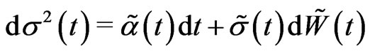
Consider the stochastic volatility model with asset price process and volatility process satisfying the stochastic differential equations

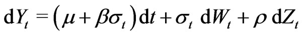(2.1)

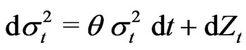(2.2)

where is a standard Brownian, , a subordinator, that is, a Levy process with only positive jumps, and are the parameters. If the model can express leverage-effect. We denote by, supported by, the Levy measure of and assume that

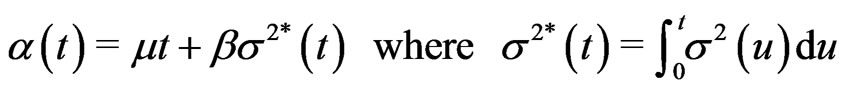
This model has been studied in [1]. The integrated volatility is defined as

(2.3)

In stochastic volatility model, calculation of conditional cummulants of the integrated volatility conditioned on the initial value is enough to be able to compute European style options.

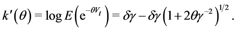
When the Levy process is an inverse Gaussian process with parameters, the cummulant functions of IGOU process are given by

We assume that the parameters of the Levy process are known. We study estimation of integrated volatility by kernel method. Observe that the realized volatility estimator is a histogram estimator of the integrated volatility where is the binwidth. Here we extend the realized volatility to include kernel weights. We take kernel weighted average of the squared increments of the observations. Our estimator includes as a special case the rolling window estimator of [2] and [3], the kernel can be chosen to satisfy the weighting schemes proposed there while the bandwidth determines the laglength. The paper also generalizes [4,5] to include weighting. The weighting scheme is jointly determined by the choice of and. With a two-sided kernel, kernel volatility (KV) takes a weighted average of the instantaneous volatility over the whole sample period. We will choose one-sided kernel.

For fixed, KV gives a weighted measure of the integrated volatility. As, we recover the instantaneous volatility at any point of continuity of.

We have the following assumptions about the kernel. Consider a continuously differentiable kernel with shrinking bandwidth. Let

(2.4)

where is a kernel which normalize to

(2.5)

For example consider the Epanechikov kernel

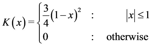(2.6)

and the kernel suggested in [6]

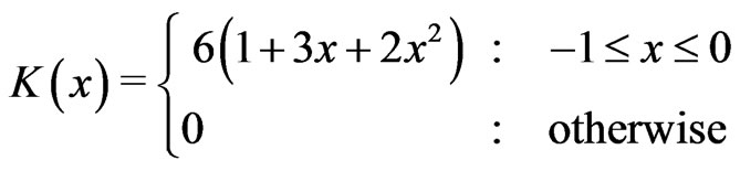(2.7)

We consider kernel weighted average of the quadratic variation. The kernel estimators converge to the integrated variance as the bandwith vanishes. In order to improve the rate of convergence of kernel estimators, we consider its relation to a moment problem.

For simplicity of notation, we will denote 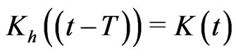and.

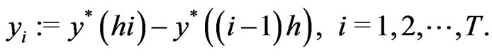
Integrated volatility has to be estimated on the basis of discrete observations of the process at times

with. Denote

(2.8)

The realized volatility is defined as

(2.9)

The following theorem is well known in the literature, see [1].

Theorem 2.1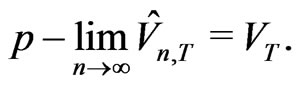

In order to improve the realized volatility with faster rate of convergence we follow the following path. The ideas are used in [7] for parametric drift estimation in diffusion processes. Define a weighted sum of squares

(2.10)

where is a weight function.

Denote

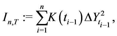(2.11)

(2.12)

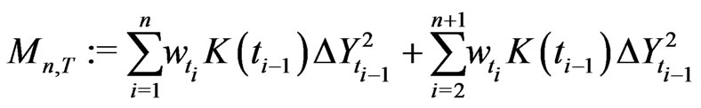
General weighted kernel volatility (KV) is defined as

(2.13)

With, we obtain the forward KV as

(2.14)

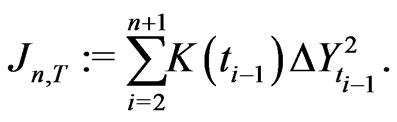
With, we obtain the backward KV as

(2.15)

[8] studied asymptotics of the estimator and obtained the rate of convergence along with asymptotic distribution of the estimator.

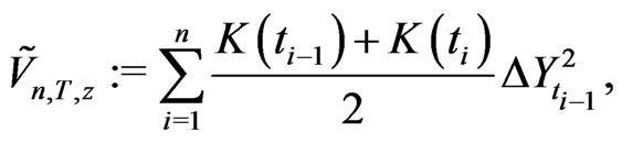
Our plan is to improve the rate of convergence by using appropriate weights for the kernel. With, the simple symmetric KV is defined as

(2.16)

With the weight function

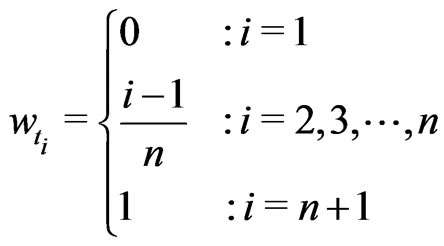
the weighted symmetric KV is defined as

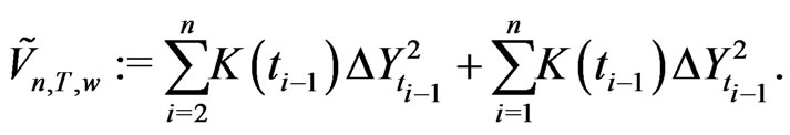(2.17)

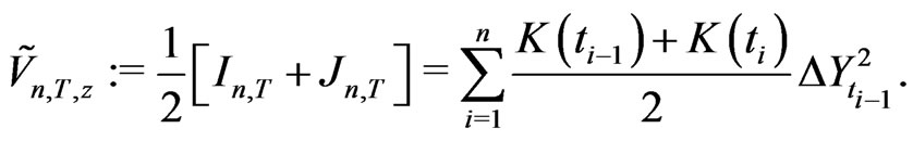
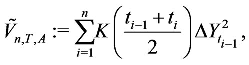
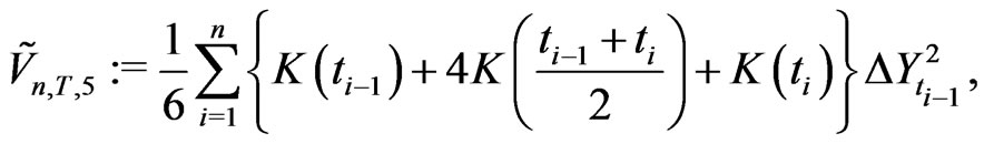
Note that estimator (2.16) is analogous to the trapezoidal rule in numerical integration. One can instead use the midpoint rule to define another estimator

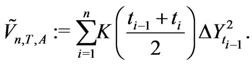(2.18)

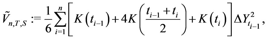
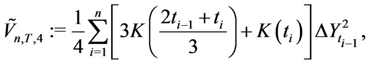
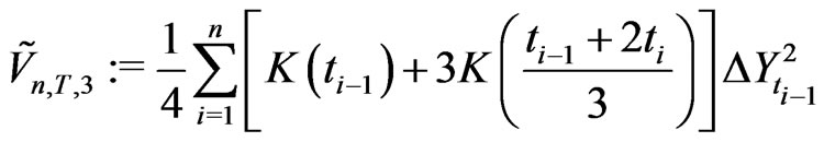
We can use the Simpson’s rule to define another estimator which is a convex combination of the midpoint estimator and the trapezoidal estimator

(2.19)

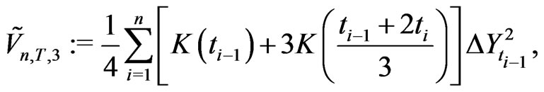
In general, one can generalize Simpson’s rule as

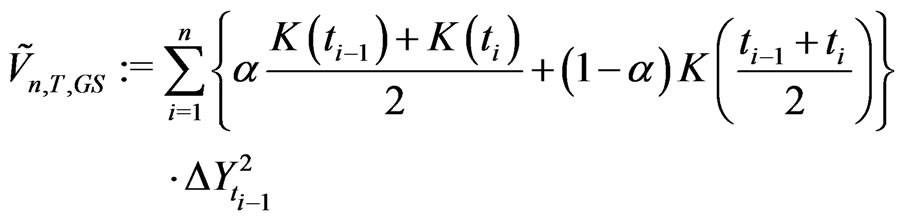(2.20)

for any.

The case produces the estimator (2.18). The case produces the estimator (2.17). The case

produces the estimator (2.19).

I propose a very general form of the quadrature based KV as

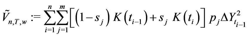(2.21)

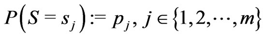
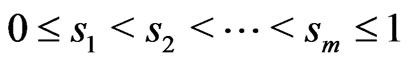where is a probability mass function of a discrete random variable on with

.

Denote the -th moment of the random variable as.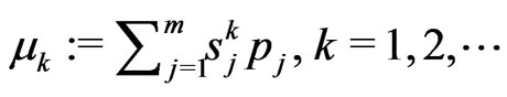

If one chooses the probability distribution as uniform distribution for which the moments are a harmonic sequence

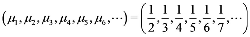then there is no change in rate of convergence than second order. If one can construct a probability distribution for which the harmonic sequence is truncated at a point, then there is a rate of convergence improvement at the point of truncation.

Given a positive integer, construct a probability mass function on such that

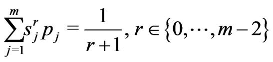(2.22)

(2.23)

Neither the probabilities nor the atoms, , of the distribution are specified in advance.

This problem is related to the truncated Hausdorff moment problem. I obtain examples of such probability distributions and use them to get higher order accurate (up to sixth order) KVs.

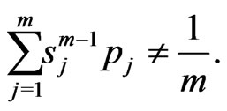
The order of approximation error (rate of convergence) of a KV is where

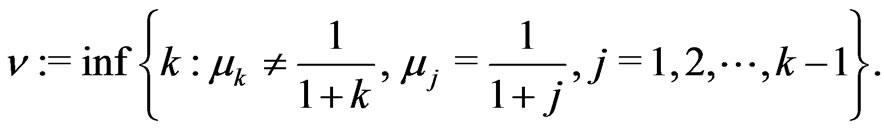(2.24)

I construct probability distributions satisfying these moment conditions and obtain KVs of the rate of convergence up to order 6.

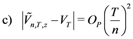
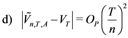
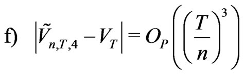
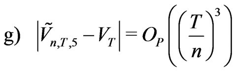
Theorem 2.2 Assume that the kernel is sufficiently smooth, continuously differentiable of order 6. The moment based estimators of integrated volatility which are given by

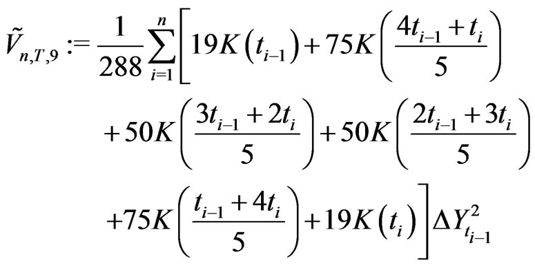
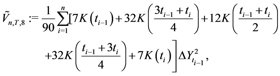
satisfy

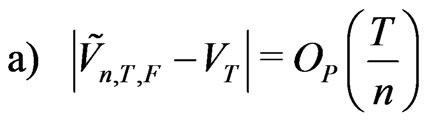
Proof We use (2.22)-(2.24). Probability at the point gives the KV (2.11) for which.

Note that. Thus. This is gives (a).

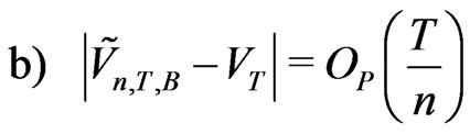
Probability at the point gives the KV(2.12) for which. Note that. Thus. This gives (b).

Probabilities at the respective points

produces the KV for which

. Thus. This gives (c).

Probability at the point produce the KV for which. Thus. This gives (d).

Probabilities at the respective points produce the asymmetric KV

(2.25)

for which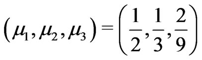. Thus. This gives (e).

Probabilities 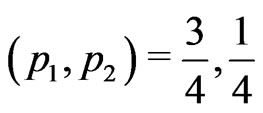at the respective points 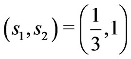produce asymmetric KV

(2.26)

for which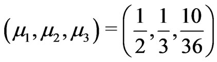. Thus. This gives (f).

Probabilities 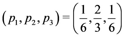at the respective points 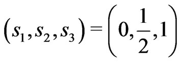produce the KV for which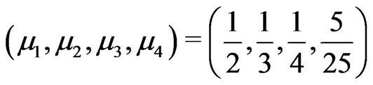. Thus.

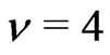This gives (g).

Probabilities 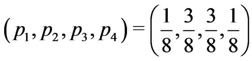at the respective points 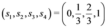produce the symmetric KV

(2.27)

for which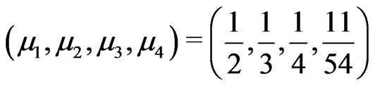. Thus.

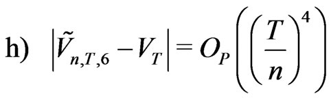
This gives (h).

Probabilities 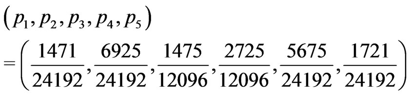at the respective points

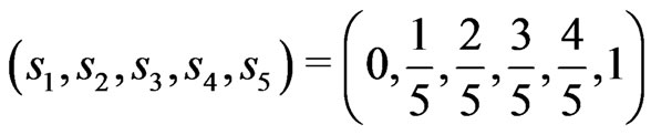
produce the asymmetric KV

(2.28)

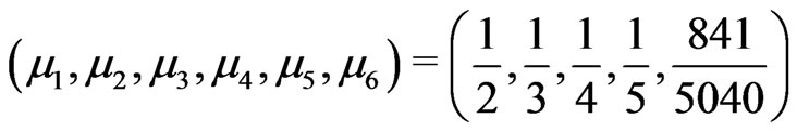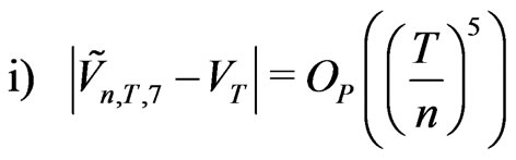
for which. Thus. This gives (i).

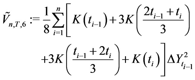
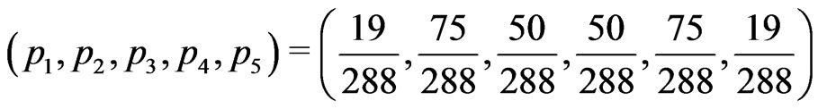
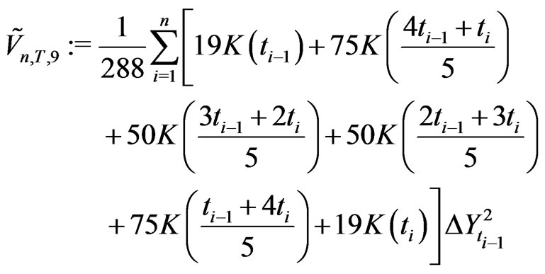
Probabilities 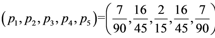at the respective points

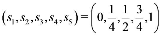
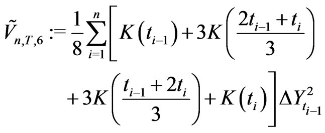
produce the symmetric KV given by

(2.29)

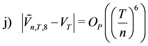
for which.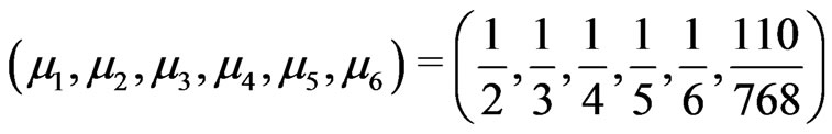

Thus. This gives (j).

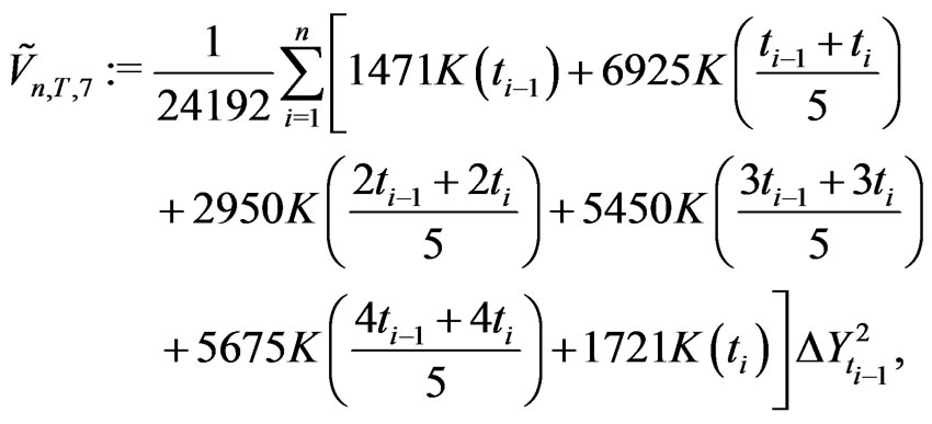
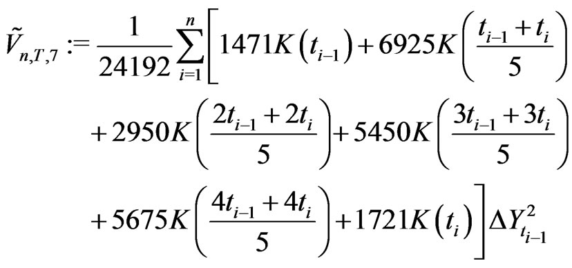
Probabilities

at the respective points

produce symmetric KV

(2.30)

for which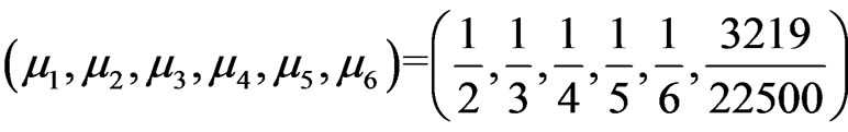. Thus. This gives (k).

The KV is based on the arithmetic mean of and. One can use geometric mean and harmonic mean instead.

Theorem 2.4 The geometric mean based symmetric KV (which is based on the ideas of partial autocorrelation) is given by

(2.31)

The harmonic mean based symmetric KV is given by

(2.32)

3. Spline Estimators

In order to improve the realized volatility estimator of integrated volatility, we use an alternative method, the method of splines, see [9], [10] and [11]. This is the first step towards the use of splines for volatility estimation. Since these are based on analysis of variance for diffusion models, we call it DANOVA models. DANOVA stands for ANOVA for Diffusions.

In the stochastic volatility model, the log-price with being the asset price, follows

where and are assumed to be independent of the standard Brownian motion. The process is called the  instantaneous volatility or  spot volatility and is called the  mean process and the Brownian motions and are allowed to be correlated. A simple example of this is

in which case is called the risk premium and is called the integrated variance.

Over an interval of time length, returns are defined as

which implies that

where

and

Here is called the  actual variance and is called the  actual mean.

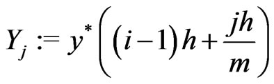
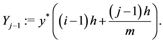
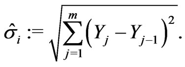
Suppose one is interested in estimating the actual volatility using intra- observations. A natural candidate is the  realized volatility given by

where

Denote

and

Thus the realized volatility is given by

When, realized volatility converges in to the integrated volatility. We consider the fixed case. The realized variance is a quadratic form.

Note that the realized volatility is based on first order difference.

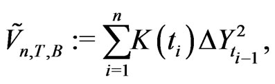
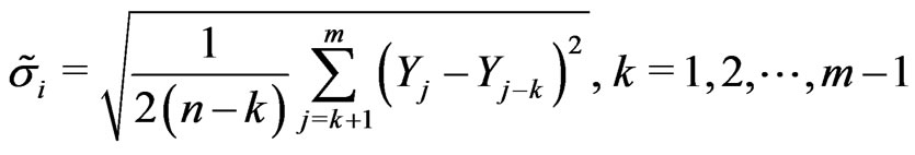
We introduce some new estimators:

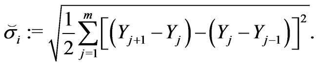
The above estimator is based on second order difference.

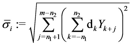
where and are non-negative integers, is called the order, and the difference sequence satisfies 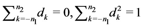and

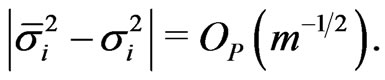
Note that for difference based estimators

To improve this error bound, we introduce the lag- estimator

In practice, the choice of the order and an appropriate difference sequence which minimizes the finite sample MSE is difficult.

Theorem 3.1 The spline estimator of integrated volatility is given by

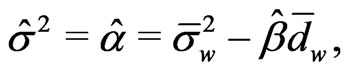
where

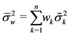
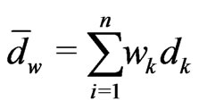
and

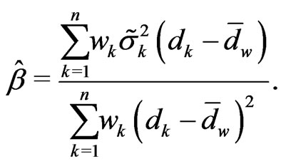
Proof We fit the following regression model:

using the weighted least squares estimate

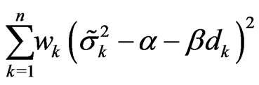
where is a sequence of i.i.d. random variables.

Let

and

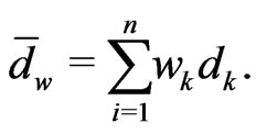
Then

where

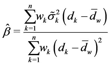
is the estimate of the intercept.

4. References

[1]    O. E. Barndorff-Nielsen and N. Shephard, “Non-gaussian Ornstein—Uhlenbeck-Based Models and Some of Their Uses in Financial Economics (with Discussion),” Journal of the Royal Statistical Society: Series B, Vol. 63, No. 2, 2001, pp. 167-241. doi:10.1111/1467-9868.00282

[2]    D. P. Foster and D. B. Nelson, “Continuous Record Asymptotics for Rolling Sampling Variance Estimators,” Econometrica, Vol. 64, No. 1, 1996, pp. 139-174. doi:10.2307/2171927

[3]    E. Andreou and E. Ghysels, “Rolling Sample Volatility Estimators: Some New Theoretical, Simulation and Empirical Results,” Journal of Business and Economics Statistics, Vol. 20, No. 3, 2002, pp. 363-375. doi:10.1198/073500102288618504

[4]    O. E. Barndorff-Nielsen and N. Shephard, “Econometric Analysis of Realised Covariation: High Frequency Based Covariance, Regression and Correlation in Financial Economics,” Econometrica, Vol. 72, No. 3, 2004, pp. 885-925. doi:10.1111/j.1468-0262.2004.00515.x

[5]    O. E. Barndorff-Nielsen and N. Shephard, “Power and Bipower Variation with Stochastic Volatility and Jumps (with Discussion),” Journal of Financial Econometrics, Vol. 2, No. 1, 2004, pp. 1-48. doi:10.1093/jjfinec/nbh001

[6]    S. Zhang and R. J. Karunamuni, “On Kernel Density Estimation near Endpoints,” Journal of Statistical Planning and Inference, Vol. 70, No. 2, 1988, pp. 301-316. doi:10.1016/S0378-3758(97)00187-0

[7]    J. P. N. Bishwal, “Parameter Estimation in Stochastic Differential Equations,” Springer-Verlag, Berlin, 2008. doi:10.1007/978-3-540-74448-1

[8]    D. Kristensen, “Nonparametric Filtering of the Realised Volatilty: A Kernel Based Approach,” Econometric Theory, Vol. 26, No. 1, 2010, pp. 60-93. doi:10.1017/S0266466609090616

[9]    C. Gu, “Smoothing Spline ANOVA Models,” SpringerVerlag, New York, 2002.

[10]    P. Hall and J. S. Marron, “On Variance Estimation in Nonparametric Regression,” Biometrika, Vol. 77, No. 2, 1990, pp. 415-419. doi:10.1093/biomet/77.2.415

[11]    G. Wahba, “Spline Models for Observational Data,” CBMS-NSF Regional Conference Series in Applied Mathematics, SIAM, Philadelphia, September 1990.