Open Journal of Geology
Vol.3 No.5(2013), Article ID:36621,9 pages DOI:10.4236/ojg.2013.35041
Microseismic Imaging of Hydraulically Induced-Fractures in Gas Reservoirs: A Case Study in Barnett Shale Gas Reservoir, Texas, USA
Mining, Petroleum, and Metallurgical Engineering Department, Faculty of Engineering, Cairo University, Giza, Egypt
Email: amabdul@miners.utep.edu
Copyright © 2013 Abdulaziz M. Abdulaziz. This is an open access article distributed under the Creative Commons Attribution License, which permits unrestricted use, distribution, and reproduction in any medium, provided the original work is properly cited.
Received July 7, 2013; revised August 7, 2013; accepted August 17, 2013
Keywords: Microseismic imaging; Barnett shale; Fracture monitoring; Unconventional reservoirs stimulations
ABSTRACT
Microseismic technology has been proven to be a practical approach for in-situ monitoring of fracture growth during hydraulic fracture stimulations. Microseismic monitoring has rapidly evolved in acquisition methodology, data processing, and in this paper, we evaluate the progression of this technology with emphasis on their applications in Barnett shale gas reservoir. Microseismic data analysis indicates a direct proportion between microseismic moment magnitude and depth, yet no relation between microseismic activity and either injection rate or injection volume has been observed. However, large microseismic magnitudes have been recorded where hydraulic fracturing stimulation approaches a fault and therefore the geologic framework should be integrated in such programs. In addition, the geometry of fracture growth resulted by proppant interactions with naturally fractured formations follows unpredictable fashion due to redirecting the injection fluids along flow paths associated with the pre-existing fault network in the reservoir. While microseismic imaging is incredibly useful in revealing the fracture geometry and the way the fracture evolves, recently several concerns have been raised regarding the capability of microseismic data to provide the fracture dimensional parameters and the fracture mechanism that could provide detailed information for reservoir characterization.
1. Introduction
Induced fracturing of hydrocarbon bearing formations has been historically documented to enhance oil and gas production for several decades since the middle of the twentieth century [1]. Nevertheless, recent activity using improved fracture stimulation has resulted in astoundingly good results in hydrocarbon production. This is contemporaneous to an exponential growth in a passive seismic imaging technology that enables mapping active fracture networks and fracture growth during hydraulic fracture stimulations [2], monitoring well failures [3], tracking injection of fluids or steam into the producing formations [4], and imaging fault networks, and rock deformation associated with reservoir compaction [5]. Of these applications, microseismic monitoring of hydraulicfracture operations for oil and gas stimulations is currently the most widely used.
Hydraulic fracturing (Figure 1) is developed to enable exposing larger drainage area to the wellbore on both vertical and horizontal well through single or multistage hydraulic fracturing techniques such as fracturing vertical well, a non-stimulated horizontal well, a single treatment horizontal hydraulic fracture, and recently Multistage horizontal wells. To better control the height and length of the induced hydraulic fractures, horizontal drilling of a well should be parallel to the minimum horizontal stress field and then hydraulically fracturing the well perpendicular to the minimum horizontal stress field. The ideal hydraulic fracture job should maintain their influence within the objective formation and prohibit penetration into the upper water-bearing interval. Ideally, the minimum horizontal stress can be determined using the structural/tectonic analysis of the developed geologic structures and/or the world stress map (www.world-stress-map.org). The down hole microseismic experiments provide the important tool to verify this direction and in consequence determine the azimuth of the horizontal track/wellbore.
Seismicity attributed to hydrocarbon production falls within two categories: induced seismicity caused by anthropogenic activity, and triggered seismicity that entails
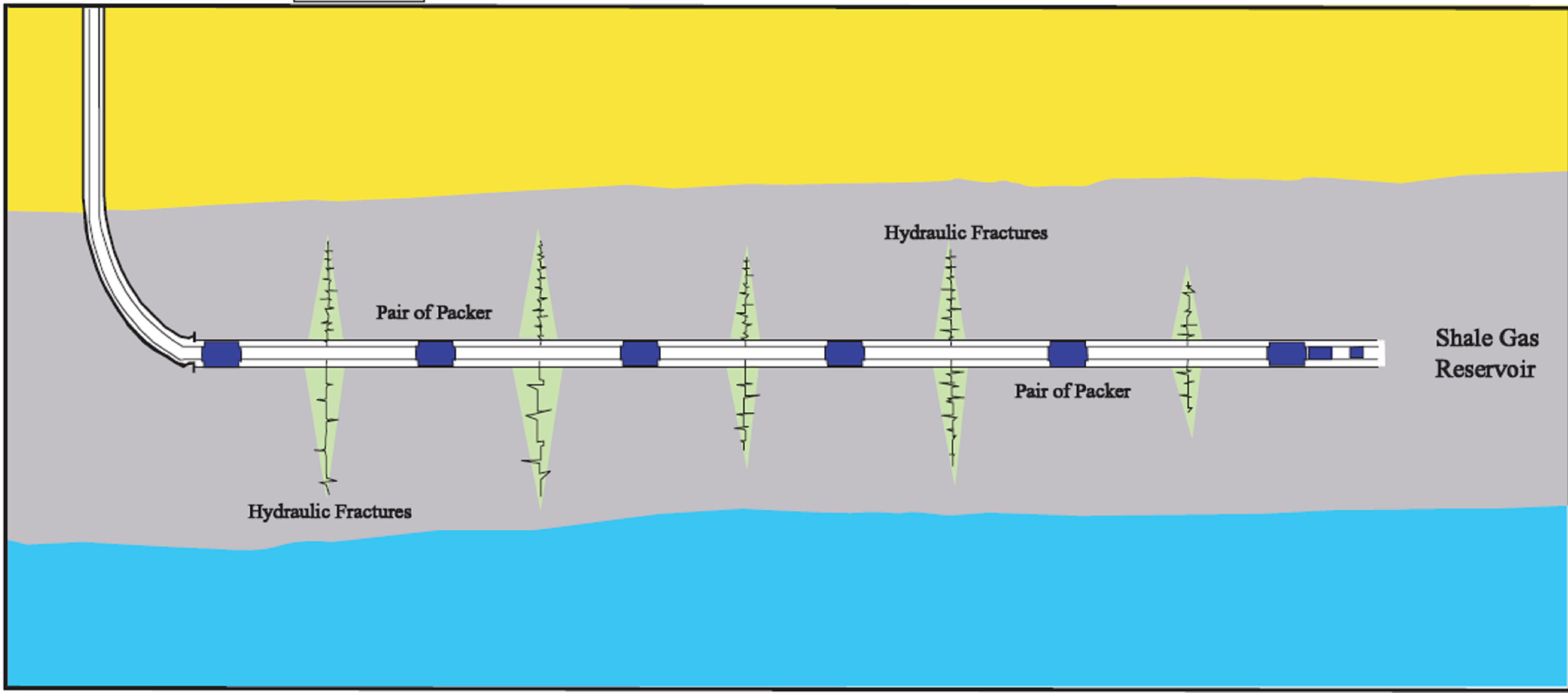
Figure 1. Multistage hydraulic fracturing through different ports separated by pairs of packers.
earthquakes whose timing is caused by anthropogenic activity [6]. Microseismic monitoring involves recording emanated elastic waves generated by microfracturing of the formation rock mass to determine the location of the micro-scale failure. To monitor microseismic events, a geophone array is installed and its location relative to the area to be monitored is accurately determined. The recorded microseismic event waveforms are amplified and validated before further processing. The event source location is calculated using the relative arrival times, the times of first break in the signal waveform, of recorded signals and the corresponding geophone locations. This is accomplished by using a suitable algorithm such as the least squares location method or the simplex method. The least squares location algorithm adopts data weighting and therefore suffers an exaggerated error effect in case of erroneous arrival times. In such a case, the simplex algorithm provides better results because it does not arbitrarily weight the data [7].
Real time intervention using microseismic monitoring during hydraulic fracturing stimulation allows effective results and minimizes the risk of seal deterioration by providing the on-site engineer with an updated image of the fracture growth. The ultimate images subsequently can be utilized in updating numerical model to simulate the predicted drainage area and enhance a better design for stimulating future wells and optimizing the fracture design. In this paper, a number of important issues entailing the technological development in microseismic data acquisition, processing, and interpretation are discussed to help understand the appropriate effective applications and potential limitations of microseismic methods. In addition, we discuss several projects that apply microseismic imaging technique in hydraulic fracturing operations in Barnett shale gas reservoir.
2. Theory
Microseismic technology follows the well established theories of the earthquake seismology and is generally characterized by very small amplitudes and relatively very high frequencies (200 - 2000 Hz). Typically microseismic detectors targets either short duration acoustic emissions related to reservoir induced deformation on pre-existing structures or the creation of new fractures during hydraulic fracturing process. Such seismic emissions are referred to as microseismicity or microseisms that may in some cases felt as small magnitude earthquake, usually lie between -1 and -3 and assumed to induce a fraction of a millimeter to millimeter in displacement or a few millimeters squared as a rupture area. Hydraulic fracturing technique uses high-pressure fluid injection to induce a decrease in the effective stress and get the Mohr’s circle of the system to touch the strength envelope. This associate a shear or tensile failure to the rock and propagation of seismic energy that can be quantified relative to the injected hydraulic energy. Reference [8] calculated the injected hydraulic energy (EH) is as;
 (1)
(1)
where PD is pressure and V is the total volume of injected fluid.
The total released energy (ER) is a function of the lithostatic stress (σl), static seismic moment (Mo) and shear modulus (μ, for typical shale reservoir is approximately 15 GPa),) and is expressed by:
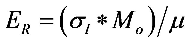 (2)
(2)
Microseismic moment (Mo) is usually determined from the recorded event’s parameters using various methods such as the simple method introduced by Brune in 1970 [9] and more sophisticated methods based on moment tensor inversion that require at least two monitoring wells [10]. In Brune method, the moment (Mo) and radius (ro) of the event is calculated from following equations Equation;
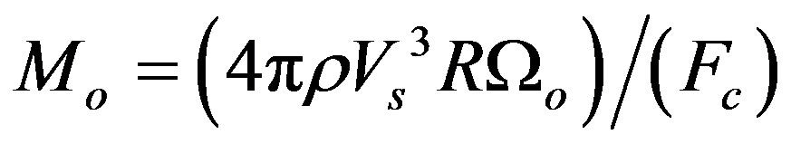 (3)
(3)
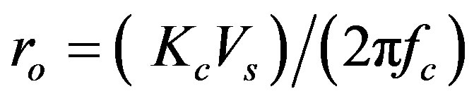 (4)
(4)
where ρ is the density (average value for shale ~2.5 gm/cc), Vs is the shear wave velocity (usually ~8000 ft/sec for typical shale), R is the receiver-event distance, Ωo is the low-frequency amplitude of the displacement spectrum, Fc is a radiation pattern factor, where Kc is a constant (~2.2), and fc is the corner frequency. A brief description of these items and the methods to obtain them is presented in Reference [11].
3. Methods
Microseismic imaging typically employs a temporary string of triaxial geophones set at eight to twelve levels in a monitoring well to evaluate the development of fracture system at the vicinity of a nearby hydraulically fractured wellbore (Figure 2). Being close to the source,
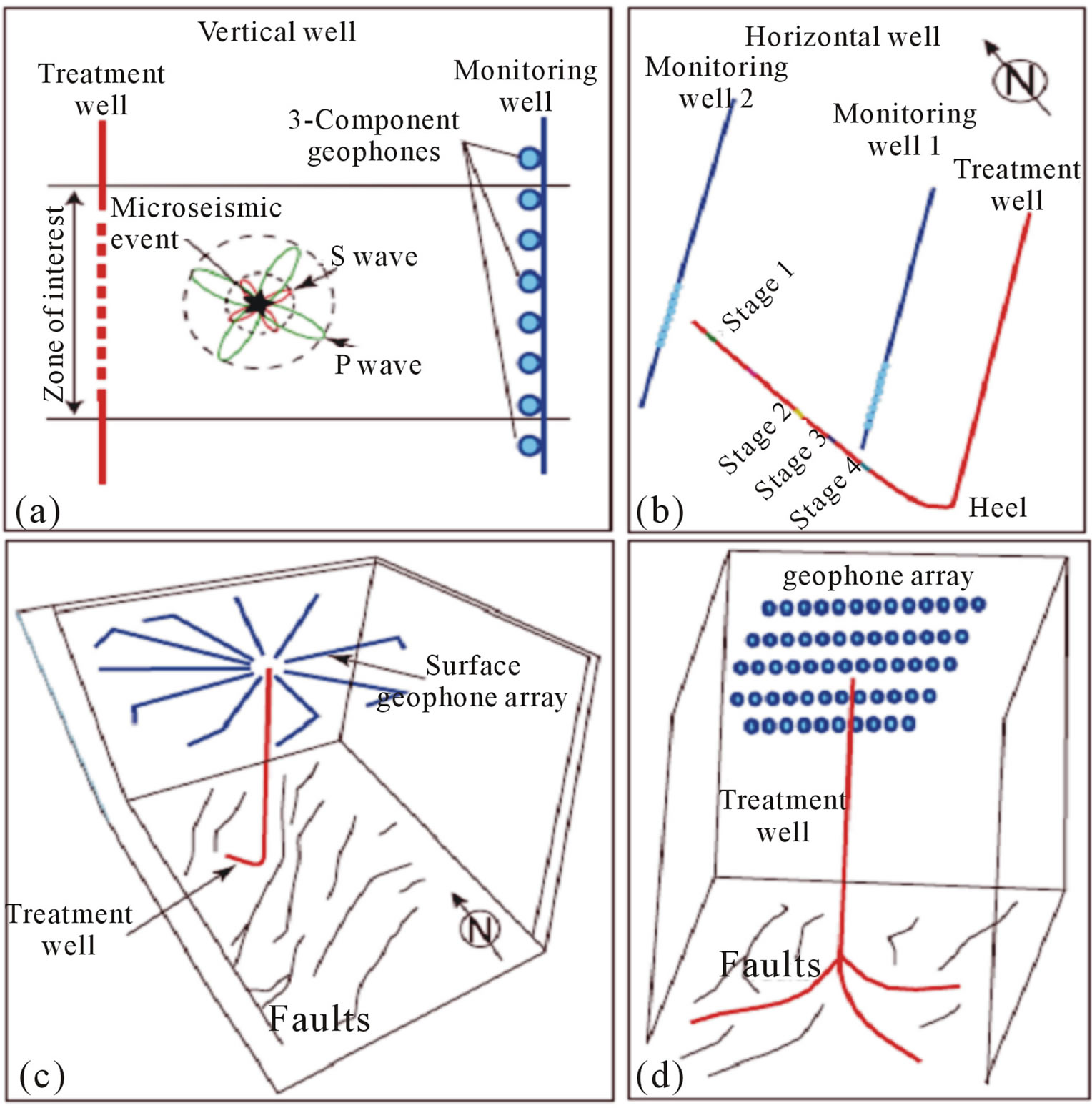
Figure 2. Data acquisition geometry of microseismic surveys. (a) 8 triaxial geophones array centered on the target formation of vertical treatment well; (b) Monitoring microseismic activity by two wells induced by hydraulic fracturing of a horizontal well; (c) Star-like surface monitoring array centered on the head of a horizontal well; (d) Surface geophone array monitoring microseismic events of a multilateral well.
signal attenuation is minimized and the signal-to-noise ratio (S/N) would be sufficient to determine the hypocenter location from the microseismic record. Furthermore, Reference [12] indicated that the prior knowledge of velocity structure can optimize the downhole geophone configuration within the available well geometry to provide a better location image. For accurate definition to the geophone placement and orientation in a vertical monitoring well, surveys including the deployment of a coil-tubing string charge in a nearby borehole are important [13]. It is a common practice in hydraulic fracturing jobs to use offset wells to install the microseismic monitoring array, but the treatment well can also be utilized for this purpose [14] with notable increase in the background noise resulting from sensors position close to the injection spot. Alternatively, near surface sensors permanently planted in a star-like (radial) or network array are usually recommended in case of hydraulic fracturing in multiple wells, continuous monitoring of a mature reservoir over long period of time, or monitoring long laterals and pad drilling over large geographical area. Near surface array are typically deployed for strategic field planning and development where monitoring wells are unavailable or comprehensive images are targeted for a large area (40 - 1300 square kilometers) over long time. Figure 3 presents the typical procedure applied in microseismic fracture monitoring for hydrocarbon production optimization and/or reservoir monitoring.
The up to 0.5 ms microseismic data is digitized downhole and transmitted through the wireline to a surface acquisition unit. The characteristics of the detected seismic signals are analyzed in an approach similar to that applied in the natural seismic events associating earthquakes. This includes calculations of pand s-wave arrival times and signal polarization that gives the way to determine the locations of events hypocenter by forward modeling of velocity structure. The arrival times of Pand S-waves is picked either manually or automatically. Automatic methods utilize one of the pseudoautomated time-picking algorithms (e.g. [15]) and subsequently checked manually for consistency. In general the location of a microseismic event using downhole data can be determined using three different categories of techniques namely; Hodogram, Triangulation, and Semblance techniques.
For a particular microseismic imaging project, the selection of the ideal technique depends on sensor configuration and the quality of the recorded data [16]. In Hodogram technique [17] data from triaxial geophones determines the direction of the hypocenter from the particle motion of the direct P-wave and/or S-wave arrivals, which is polarized in the direction of propagation under certain conditions. The event distance is calculated from the velocity and the difference in arrival time of direct P-
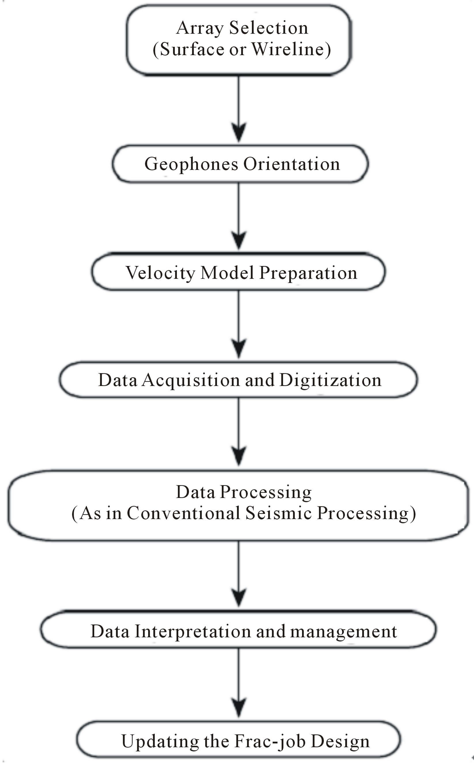
Figure 3. Typical steps applied in microseismic fracture monitoring.
and S-waves emanated from this event. Reliable hypocenter location is obtained using hodograms of multiple recording location and detailed velocity model of the investigation site. In triangulation technique (e.g. [18]) arrival times of Pand/or S-waves combinations at multiple stations in a triangulation scheme are used. This arrival times together with the velocity model determine the distance of the microseismic event relative to the monitoring well. In Semblance technique (e.g. [19]) a single phase arrival, applied in large aperture array, or multiple phases arrivals , suitable for small aperture of the downhole arrays, are utilized to determine a point in the space, correspond to the hypocenter location, that maximize the semblance measure. Semblance technique does not depend on discrete arrival times to image the source location and therefore is conceptually similar to Kirchhoff migration.
Technical Considerations
For most microseismic projects, the main technical challenge is to obtain a sufficient sensitivity of the deployed array that enables acquisition of sufficient microseismic signal strength relative to the acoustic/electronic noise. The number of recordable low amplitude events depends on the nature and magnitude of the background noise and transmission losses that vary depending on the sourcedetector separating distance and the mechanical properties of the medium. Typically, source moment magnitudes in the range (–3 Mw) to (–1 Mw) can be recorded as strong events in hydraulic fracturing operations [20] and if the source-receiver offset is relatively large (~ 800 m or more) these events could be only recorded over the natural earth background. Additional complications may arise due to impulsive acoustic noise associating the ordinary operations in oil fields such as noise for borehole, pumps, and on land surface activities but most of this noise can be eliminated in the early stages of data processing. Normally, coherent noise can be categorized based on signal attributes or apparent moveout across the seismic array but the background seismic noise always vary from site to site.
The quality of a microseismic image depends on the uncertainty of locating the hypocenter of events; commonly refer to as resolution. This uncertainty accounts for two types of quantifiable data errors; random data errors, due to uncertainties in arrival time and hodogram data, and systematic data errors that occur as a result of inaccurate geometrical configuration and/or a simplified velocity model. Random errors tends to show “blurring” above and below the target unit if the depth errors is considerably larger than the thickness of that layer while systematic errors from velocity model lead to erroneous depth of the events. Further, Systematic errors arising from geometrical uncertainties, the actual location of sensors in a borehole, induce systematic offsets in the image that is difficult to identify due to the exaggerated drilling and surveying accuracies. Therefore, a great caution should be considered while interpreting the spatial and temporal elements of a microseismic image particularly in case of locating seismic events within thin layers.
The spatial distribution of the events identified microseismic image is usually sporadic and erratic which makes a unique identification of the induced fracture patterns almost impossible. Analogous to earthquake seismology, the techniques applied to identify significant geologic structures from earthquakes cloud (e.g. [21]) can be exploited in identifying the fracture geometrical pattern from the microseismic cloud (e.g. [4]). In addition, Clustering and collapsing algorithms have been utilized to suppress the spreading the originally coherent events (e.g. [22]). Reference [23] estimated the stimulated reservoir volume (SRV) by the shape analysis of microseismic events cloud in three dimensions, but this imply equal events weightings and in consequence the estimated SRV represents the optimum value.
4. Barnett Shale Reservoir
The Barnett Shale represents one of the most active gas reservoirs in the United States with approximately 500 feet thick encountered at 6500 ft to 8000 ft depth in Fort Worth basin, North Texas [24]. It is a Mississippian-age, organic-rich, marine shale with fine grained nonsiliclastic shelf deposits that unconformably overlies Ordovician rocks (Figure 4) [25]. The Barnett formation provides the source rock, the reservoir rock and the seal for the present reservoir core samples from taken Wise County test well showed the average porosity 3.5%, very low permeability (0.001 to 0.00009 millidarcy), water saturation 40% - 50% and at least 75% of all natural fractures were filled with carbonate cement. Typical composition of the Barnett is 2% - 8% organics, 20% - 30% clay minerals (illite), 45% - 55% silt sized quartz and feldspar, 15% - 19% carbonates and trace amounts of siderite and pyrite. Barnett shale is naturally densely fractured with very low permeability and large fracture network developed perpendicular to the direction of maximum horizontal stress; the direction of development of fractures by stimulation [26]. For highly successful fracturing operations the horizontal well must be contained within the Upper and Lower Barnett Shale (Figure 4). Throughout most of the productive area, the Viola limestone separates the underlying, water-bearing Ellenberger formation from the Barnett Shale formation and behaves as the lower barrier to hydraulic fracturing [27] but it pinches out to the west and southwest (Figure 4).
Technological advancements in shale Gas stimulations have raised recovery of initial gas inplace (GIP) of Barnett Shale from 2% in 1998 to over 50% recovery in 2008 and in general the Expected Ultimate recovery is expected to be in the 15% to 35% range, depending on the nature of shale, completion technique and operator [28]. Over the last decade, over 1100 microseismic experiments are completed in the Barnett formation that elucidated numerous information about the natural/hydraulic fracture systems and identified the relationship between flow path generation and stimulation parameters. Conventional hydraulic-fracture models usually adopt the development of a single fracture, however the complex fracture network of different orientations, as found in Barnett shale, have been recognized in the early microseismic projects (e.g. [5]). This significantly alter the drainage architecture compared to the original proposed design and in consequence microseismic images integration with the hydraulic fracture models have proven to be fundamental component for production optimization.
Reference [5] analyzed the hypocenters associated the fracture growth in Barnett shale during several hydraulic fracturing treatments and notice inconsistent microseismmic images in the area around the treatment wells. Such inconsistency motivated correlating microseismic data with the hydraulic treatment parameters to infer the fluidrock interaction and estimate the treatment efficiency. Therefore, the microseismic activity within certain time window indicates the behavior of fracture length generated by the placement of proppant and/or the injected fluid. For example, Reference [29] related the instantaneous diminution in fracture length to a partial blockage induced by high proppant concentration in the frac fluid that may develop to a complete blockage and completely prevent further fluid injections into the formation. This can be traced on the microseismic image as a decrease or even cease in microseismicity at the proximity of the blockage site and a subsequent rejuvenation in seismicity reveals blockage dissolution with instantaneous growth in fracture length. This indicates that in case of fracture growth by proppant interaction with the natural fractural network, the geometry of the stimulated fractures follows unpredictable fashion as a result of redirection of fluids along characteristic fluid-flow paths associated with the fault network in the reservoir ([30]).
Knowledge of the fault plane orientation proved critical to microseismic data interpretation as energy radiation patterns from the source are highly asymmetric and as a result unique interpretation from different monitoring angles relative to the slippage almost impossible. Reference [22] showed that source parameters interpretation of microseismic data in Cotton Valley experiment was misleading due to neglecting of radiation-pattern effects. This information is highly important to understanding the prevalent fracturing process and calculations of the fracture parameters including fracture area, displacement, and slippage that appear critical for the ability to place proppant. To accurately interpret microseismic data for such information, two monitoring wells with large arrays with good quality data from most levels (at least 5) are required. Unfortunately few microseismic experiments in Barnett reservoir utilize two monitoring wells. A record of these wells (Figure 5) was available to the present work for reevaluation in which approximately 30% of the recorded events was selected for detailed interpretation using moment-tensor inversion method described by Reference [31]. To recognize approximate radiation pattern of the microseismic energy a plot of the S/P ratio against the azimuthal position of approximately 100 good events is constructed and a theoretical solution is overlained on (Figure 6). In addition the geometrical patterns of the developed fracture system was determined (Figure 7) and showed that the majority of fractures follow N 35˚ E to N 50˚ E strike with dominant slippage towards the SE. The majority of the developed fracture fall within 10˚ - 20˚ from the vertical with few events exceeds 40˚. This geometry coincides greatly with the structure orientations recorded in the Barnett shale reservoir [5]. As shown in Figure 5, the trajectory of the horizontal well is nearly perpendicular to the azimuth of the induced fractures, which in turn provide the maxi-
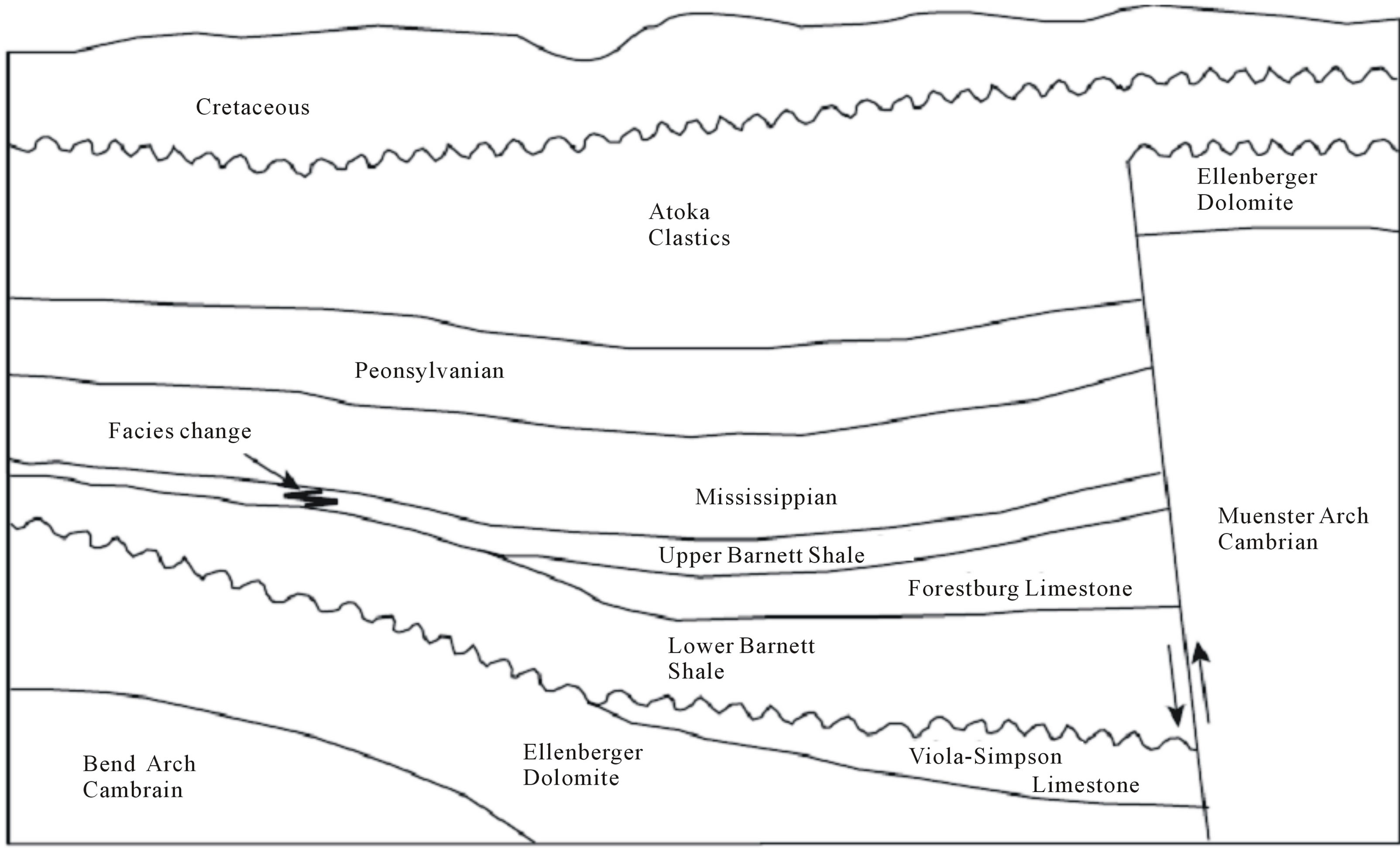
Figure 4. Geologic cross section in Fort Worth basin, North Texas.
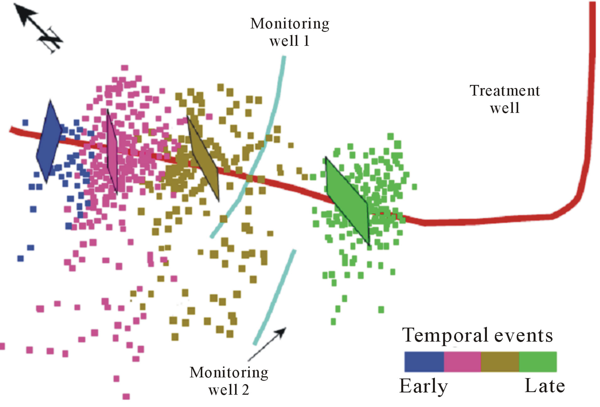
Figure 5. Microseismic imaging of induced fractures developed 4 stage hydraulic fracturing in Barnett shale gas reservoir with events temporally color. Inclined rectangles overlay indicate the dominant fracture orientation interpreted from SMT inversion.
mum drainage area to the stimulated reservoir volume. In addition the fracture height is relatively deviated upward from the symmetrical position around the horizontal borehole to avoid fracture propagation into the underlying aquifer of Ellenberger formation.
5. Discussion
The seismic moment tensor (SMT), a parameter that describes the fracture behavior at the seismic source, has been utilized in the microseismic imaging to help understanding the fracture growth (e.g. [32]). Compared to earthquake seismology that successfully utilizes seismic moment tensor inversion, the good estimation of moment tensor during hydraulic fracturing operation, even with multiple monitoring wells, remain problematic [11]. For different source mechanism (strike slip, shear, and a mix strike slip-shear), Reference [33] constructed a plot of S/P amplitude ratio of high signal-to-noise ratios signals from different hydraulic fracturing projects at various sites using the azimuth relative to the trend of the main microseismic cloud. Results of the present SMT inversion analysis (Figure 6) showed that the energy propagation fit strike-slip shear mechanism, particularly at high S/P ratios, to shear mechanism that probably dominates the lower S/P ratios with a relative symmetry around S nodal and a good match in low amplitude ratios. In addition, high S/P amplitude ratios are noticed to predominate if shear was the main microseismic mechanism in the selected projects [33]. Actually, despite the fact that S/P amplitude ratio plot does not full moment tensor inversion, but it reflects the nature of directional coverage of the radiation pattern and enables qualitatively the assessment of match between the mechanism model and the observed data.
The moment tensor and direction records in micro-
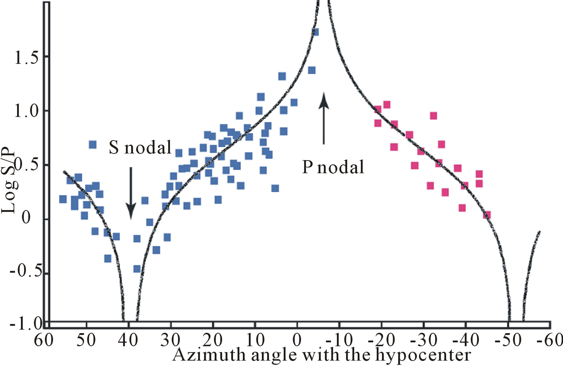
Figure 6. Plot of azimuthal position versus log S/P ratio of the events with overlay of the optimized theoretical solution for the radiation pattern that fit the microseismic events in Barnett shale gas reservoir.
seismic data enable describing the fracture mechanism mathematically by pairs of dipoles acting on the fracture plane in opposite directions. Geomechanical interpretation and fracture orientation is practically obtained by SMT inversion of source radiation pattern (Figure 6 and 7) which adopts different modes of failure [34]. This helps to understand the evolution the fracture network geometry including the fracture expansion/blockage through the overlapping hydraulic frac stages [35], recognizing the regions of diminished return [36]. Such information not only improves reservoir simulation but also optimizes the treatment economics [29]. However, Reference [11] indicated that while microseismic imaging is incredibly useful in revealing the fracture geometry and the way the fracture evolves but it does not provide detailed information about the fracturing process (mechanism) and seems currently with limited value for reservoir characterization.
Several methods have been developed to calculate the moment of microseismic events which fall within two categories: the simple methods such as Brune moment calculation [9] and sophisticated methods that use moment tensor inversion to obtain the full moment tensor and high-quality data to get accurate information but require two monitor wells (e.g. [9]). In a comparison between the magnitude calculations between the two methods, Reference [11] indicated a good agreement between the Brune spectral analysis and the moment tensor inversion, despite the considerable scatter plot, with overall Brune magnitudes less than the moment tensor inversion. This is attributed to disability of spectral analysis to fully consider the radiation pattern and non-shear behavior. Generally, most microseismic events magnitudes in typical shale reservoir fall within -0.5 and -3 Mw but relatively large events 1.0 Mw if the hydraulic treatment approached a fault plane which lead Reference [33] consider hydraulic fracturing as aseismic events.
SRV is usually calculated using the dimensions of the 3D seismic cloud that is commonly associated with both measurement uncertainty and tendency towards over SRV estimations [37]. Through early evaluations of the relationship between the measurement uncertainty and the volume of microseismic cloud, Reference [38] indicated that larger source location uncertainty is associated with the larger the microseismic cloud volume with a tendency to overestimate the underlying deforming volume. The tendency towards SRV overestimated develops due to the microseismicity induced by stresses of hydraulic treatment acting on pre-existing structures, which is usually not represented in geomechanical models [6]. Despite this drawback, microseismic images are capable of depicting complex and more sophisticated fracture models that simulate composite interactions between the hydraulic stress and original fracture systems compared to those produced from geomechanical analysis. Post hydraulic fracture production rates and reservoir drainage should intuitively be comparable to the microseismic estimates of SRV; however the disability of microseismic imaging to differentiate between the seismicity induced by fracture opening and closure remains the principle explanation for such discrepancy. In addition, the ultimate permeability within the estimated SRV is usually greatly diminished as the recorded seismicity is typically proportional to the volume of the induced fracture that is mostly partially filled with the proppant and finally the overall fracture volume is dramatically reduced by releasing the pressurized injection fluids as the well is put on production. Similarly, the geomechanical models do not consider the effect of proppant in the estimates of the ultimate fracture volume but, the microseismic images can be used to calibrate the hydraulic dimension against a complex fracture model [39].
6. Conclusion
Recently, microseismic imaging has been proven to be influential to the success of hydraulic fracturing operations in tight hydrocarbon reservoir, particularly gas reservoir. In addition, it improves the understanding of important processes in reservoir level through detailed and sometime real time changes in reservoir architecture that could be a key factor in adjusting both stimulation and drilling strategies. This is clearly manifested in Barnett shale gas reservoir that is 10 years ago among unconventional tight reservoir and today is one of the important natural gas sources in the United States. Despite the great success in fracture monitoring, microseismic technology still need to incorporate several geometrical parameters of the developed fracture system to be integrated to reservoir simulation. Such information not only improves reservoir management but also optimizes the treatment economics.
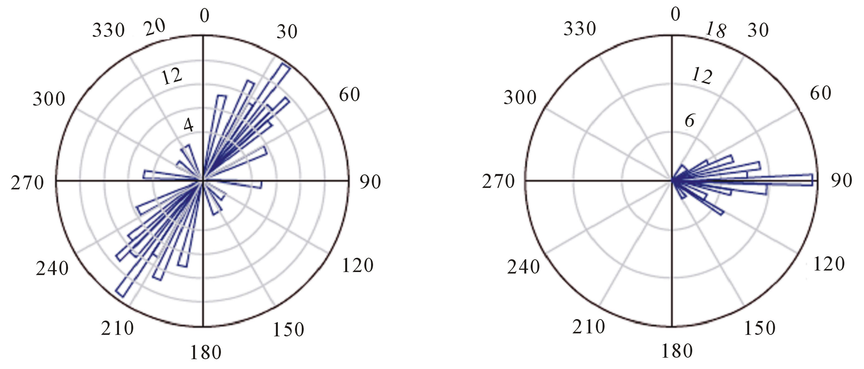
Figure 7. Strike (left) and dip (right) plot for the slippage planes of the important events in figure 5 that appears to follow the dominant trends in Barnett shale of North Texas.
7. Acknowledgements
The author would like to acknowledge the hard work of many anonymous geophysicists and field crews for acquiring and processing the utilized data.
REFERENCES
- J. B. Clark, “A Hydraulic Process for Increasing the Productivity of Oil Wells,” AIME Transactions, Vol. 186, No. 1, 1949, pp. 1-8.
- A. J. Caley, J. M. Kendall, R. H. Jones, O. I. Barkved and P. G. Folstad, “Monitoring Fractures in 4D Using Microseismic Data,” EAGE 63rd Conference and Technical Exhibition, Amsterdam, 1-15 June 2001.
- T. J. Boone, S. Nechtschien, R. Smith, D. Youck and S. Talebi, “Microseismic Monitoring for Fracturing in the Colorado Shales above a Thermal Oil Recovery Operation, in Rock Mechanics for Industry,” The 37th US Symposium on Rock Mechanics (USRMS), Vail, 7-9 June 1999, pp. 1069-1076.
- S. C. Maxwell, T. Urbancic, M. Prince and C. Demerling, “Passive Imaging of Seismic Deformation Associated with Steam Injection in Western Canada,” Proceedings of Society of Petroleum Engineers Annual Technical Conference, Denver, 5-8 October 2003.
- S. C. Maxwell, T. Urbancic, N. Steinsberger and R. Zinno, “Microseismic Imaging of Fracture Complexity in the Barnett Shale,” Proceedings of Society of Petroleum Engineers Annual Technical Conference, San Antonio, 29 September-2 October 2002.
- S. C. Maxwell, M. Jones, R. Parker, S. Leaney, M. Mack, D. Dorvall, D. D’Amico, J. Logel, E. Anderson and K. Hammermaster, “Fault Activation during Hydraulic Fracturing,” Proceeding of the 79th Society of Exploration Geophysicists International Exposition and Annual Meeting 2009, Houston, 25-30 October 2009.
- J. Riefenberg, “A Simplex Method-Based Algorithm for Source Location of Microseismic Events Associated with Underground Mining,” The 30th US Symposium on Rock Mechanics (USRMS), Morgantown, 19-22 June 1989.
- J. F. Gibbs, J. H. Healy, C. B. Raleigh and J. Coakley, “Seismicity in the Rangely, Colorado, Area: 1962-1970,” Bulletin of the Seismological Society of America, Vol. 63, No. 5, 1973, pp. 1557-1570.
- J. N. Brune, “Tectonic Stress and the Spectra of Seismic Shear Waves from Earthquakes,” Journal of Geophysical Research, Vol. 75, No. 26, 1970, pp. 4997-5009. doi:10.1029/JB075i026p04997
- R. C. Nolen-Hoeksema and L. J. Ruff, “Moment Tensor Inversion of Microseisms from the B-Sand Propped Hydrofracture, M-Site, Colorado,” Tectonophysics, Vol. 336, No. 1-4, 2001, pp. 163-181. doi:10.1016/S0040-1951(01)00100-7
- N. R. Warpinski, J. Du and U. Zimmer, “Measurements of Hydraulic-Fracture-Induced Seismicity in Gas Shales,” SPE Hydraulic Fracturing Technology Conference, Woodlands, 6-8 February 2012.
- D. Raymer, Y. Ji, R. Behrens and J. Ricketts, “Genetic Algorithm Design of Microseismic Injection-Monitoring Networks in the Tengiz Field,” 74th SEG Annual International Meeting, Denver, 10-15 October 2004, pp. 548- 551.
- P. Bulant, L. Eisner, I. Psencik and J. Le Calvez, “Importance of Borehole Deviation Surveys for Monitoring of Hydraulic Fracturing Treatments,” Geophysical Prospecting, Vol. 55, No. 6, 2007, pp. 891-899. doi:10.1111/j.1365-2478.2007.00654.x
- E. Gaucher, C. Maisons, E. Fortier and P. Kaiser, “Fracture Mapping Using Microseismic Monitoring Data Recorded from Treatment Well—Results Based on 20 Hydro-Fracturing Jobs,” 67th EAGE Conference & Technical Exhibition, Madrid, 13-16 June 2005.
- J. Drew, D. Leslie, P. Armstrong and G. Michaud, “Automated Microseismic Event Detection and Location by Continuous Spatial Mapping,” 2005 SPE Annual Technical Conference & Exhibition, Dallas, 9-12 October 2005.
- G. Pavlis, “Appraising Earthquake Hypocenter Locations Errors: A Complete Practical Approach for Single Event Locations,” Bulletin of the Seismological Society of America, Vol. 76, No. , 1986, pp. 1699-1717.
- J. N. Albright and R. J. Hanold, “Seismic Mapping of Hydraulic Fractures Made in Basement Rocks,” Proceedings of the Energy Research and Development Administration-ERDA-Symposium on Enhanced Oil and Gas Recovery, Tulsa, 9-10 June 1976.
- S. J. Gibowicz and A. Kijko, “An Introduction to Mining Seismology,” Academic Press Inc., New York, 1994.
- S. Rentsch, S. Buske, S. Luth and S. A. Shapiro, “Fast Location of Seismicity: A Migration-Type Approach with Application to Hydraulic-Fracturing Data,” Geophysics, Vol. 72, No. 1, 2007, pp. S33-S40. doi:10.1190/1.2401139
- S. C. Maxwell, “A Brief Guide to Passive Seismic Monitoring,” 2005 CSEG National Convention, Calgary,16-19 May 2005.
- R. Jones and R. C. Stewart, “A Method for Determining Significant Structures in a Cloud of Earthquakes,” Journal of Geophysical Research, Vol. 102, No. B4, 1997, pp. 8245-8254.
- J. T. Rutledge and W. S. Phillips, “Hydraulic Stimulation of Natural Fractures as Revealed by Induced Microearthquakes, Carthage Cotton Valley Gas Field, East Texas,” Geophysics, Vol. 68. No. 2, 2003, pp. 441-452. doi:10.1190/1.1567214
- M. J. Mayerhofer, E. P. Lolon, N. R. Warpinski and C. L. Cipolla, “What Is Stimulated Reservoir Volume (SRV)?” Shale Gas Production Conference, Fort Worth, 16-18 November 2008.
- S. C. Maxwell, “Microseismic: Growth Born from Success,” The Leading Edge, Vol. 29, 2010, pp. 338-343. doi:10.1190/1.3353732
- S. L. Montgomery, D. M. Jarvie, K. A. Bowker and R. M. Pollastro, “Mississippian Barnett Shale, Fort Worthbasin, Northcentral Texas: Gas-Shale Play with Multi-Trillioncubic Foot Potential,” AAPG Bulletin, Vol. 89, No. 2, 2005, p. 155. doi:10.1306/09170404042
- L. Mathews, G. Schein and M. Malone, “Stimulation of Gas Shales: They’re All the Same-Right?” SPE Hydraulic Fracturing Technology Conference, College Station, 29- 31 January 2007.
- J. H. Le Calvez, R. C. Klem, L. Bennett, A. Enwemi, M. Craven and J. C. Palacio, “Real-Time Monitoring of Hydraulic Fracture Treatment: A Tool to Improve Completion and Reservoir Management,” SPE Hydraulic Fracturing Technology Conference, College Station, 29-31 January 2007.
- G. E. King, “Thirty Years of Gas Shale Fracturing: What Have We Learned?” SPE Annual Technical Conference and Exhibition, Florence, 19-22 September 2010.
- S. Maxwell, T. Urbancic, J. H. Le Calvez and W. D. Grant, “Passive Seismic Imaging of Hydraulic Fracture Proppant Placement,” SEG Expanded Abstracts, Vol. 23, 2004, p. 560. doi:10.1190/1.1851294
- A. Wuestefeld, T. Urbancic, A. Baig and M. Prince, “After a Decade of Microseismic Monitoring: Can We Evaluate Stimulation Effectiveness and Design Better Stimulations,” SPE/EAGE European Unconventional Resources Conference and Exhibition, Vienna, 20-22 March 2012.
- N. R. Warpinski and J. Du, “Source-Mechanism Studies on Microseismicity Induced by Hydraulic Fracturing,” SPE Annual Technical Conference and Exhibition, Florence, 19-22 September 2010. doi:10.2118/135254-MS
- A. Baig and T. Urbancic, “Microseismic Moment Tensor: A Path to Understand Frac Growth,” The Leading Edge, Vol. 29, 2010, pp. 320-324. doi:10.1190/1.3353729
- S. C. Maxwell, M. Jones, D. Cho and M. Norton, “Understanding Hydraulic Fracture Variability through Integration of Microseismicity and Seismic Reservoir Characterization,” 46th US Rock Mechanics/Geomechanics Symposium, Athens, Chicago, 27-30 March 2011.
- S. Leaney and C. Chapman, “Microseismic Sources in Anisotropic Media,” 72nd EAGE Conference & Exhibition Incorporating SPE EUROPEC 2010, Barcelona, 14- 17 June 2010.
- A. Baig, T. Urbancic, K. Mace and M. Prince, “Assessing the Spacing of Stages in Plug-and-Perf Completions through Seismic Moment Tensor Inversion,” SPE Hydraulic Fracturing Technology Conference, The Woodlands, 6-8 February 2012.
- K. Mace, T. Urbancic and A. Baig, “Fracture Treatment Optimization Via Points of Diminishing Returns as Determined by Seismic Moment Tensor Inversion,” Canadian Unconventional Resources Conference, Calgary, 15- 17 November 2011.
- S. C. Maxwell, “What Does Microseismic Tell Us about Hydraulic Fractures?” 2011 CSGP CSEG CWLS Convention, San Antonio, 18-23 September 2011.
- S. C. Maxwell, B. Underhill, L. Bennett and A. Martinez, “Key Criteria for a Successful Microseismic Project,” 2010 SPE Technical Conference, Florence, 19-22, September 2010.
- C. L. Cipolla, M. J. Williams, X. Weng, M. Mack and S. C. Maxwell, “Hydraulic Fracture Monitoring to Reservoir Simulation: Maximizing Value,” 2010 SPE Technical Conference, Florence, 19-22, September 2010.