Open Journal of Geology
Vol. 2 No. 3 (2012) , Article ID: 21386 , 10 pages DOI:10.4236/ojg.2012.23015
Numerical Analyses of Seepage from Behesht Abad Dam Foundation
Geology Department, The University of Isfahan, Isfahan, Iran
Email: ameneh.dardashti@yahoo.com, rasajl@ui.ac.ir
Received March 25, 2012; revised April 26, 2012; accepted May 11, 2012
Keywords: Hydraulic aperture; Hydro-mechanical behavior of joints; Mechanical aperture; Numerical analyses; Seepage
ABSTRACT
In this article, seepage phenomena through the Karstic limestone foundation of Behesht Abad dam are investigated. In order to get a state of seepage and determine the depth of grouting curtain, it has been tried to evaluate the seepage of Behesht-Abad dam foundation and its abutments by the help of numerical analysis and UDEC 4.0 software. To perform this research, firstly, geological data during a study phase in Behesht Abad dam site was gathered, and then different methods have been used to calculate the engineering properties of rock mass. Therefore the structural model of dam foundation based on the geological data constructed and various boundary conditions including different heads were applied on the model and the suitable depth for the grouting curtain was proposed.
1. Introduction
Dams are such structures that constructed to control and store surface water. The main reasons for constructing of Behesht-Abad Dam are the existence of important Industries in the Zayandeh Rood basin, growing population in this area and growing the need of water in central part of Iran. So, transferring water from a part of Karoon basin (Behesht-Abad region) to the center of Iran has been proposed. In each dam construction project, seepage analysis in foundation and abutments for designing the suitable curtain is one of the most important parts of projects. The most common method to evaluate the permeability of rock mass is water pressure tests. By help of this method, permeability of foundation and abutments, hydro-mechanical behaviors and the seepage potential has been examined. The performed water pressure tests indicate the necessity of providing a grout curtain below the Behesht Abad dam foundation.
In this regard, Lugeon values and also the hydro-mechanical behavior of investigation boreholes are calculated and their frequencies in each part have been assigned. The situation of investigation boreholes are shown in Figure 1.
Numerical analysis methods have been using in engineering projects for a long time, but using of these methods for seepage analysis of rock mass isn’t that much old. UDEC has the capability to perform the analysis of fluid flow through the fractures of a system of impermeable blocks. A fully coupled mechanical-hydraulic analysis is performed, in which fracture conductivity is dependent on mechanical deformation and, conversely, joint water pressures affect the mechanical computations. Both confined flow and flow with a free surface can be modeled in UDEC. In these methods, structural model of dam and its foundation based on geological Data is designed in the software, and then seepage and fluid flow through rock joints are studied, by implementation of different water pressure behind dam.
Among all available software, UDEC is a two-dimensional software which is designed based on distinct element methods and is used for discontinuous environments modeling. UDEC was originally developed to perform stability analysis of jointed rock slopes. This software modelizes the discontinuous environments like jointed rock in static and dynamic situations. It's capable of analysis the fluid flow from joint sets and cracks of impermeable blocks system. These analyses are the hydraulic ones. It means that the hydraulic conductivity of joints directly depends on mechanical deformations, and vice versa the water pressure of joints affects the mechanical calculations.
UDEC is based upon a command-driven format. Word commands control the operations of the program. This is an important distinction. The command-driven structure allows UDEC to be a very versatile tool for use in engineering analysis. However, this structure can present difficulties for new or occasional users. There are over
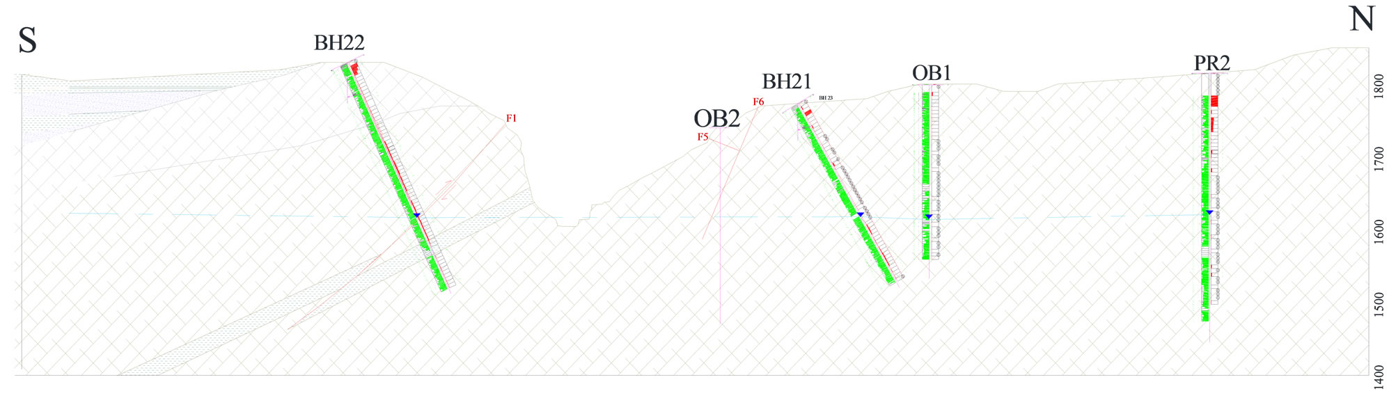
Figure 1. The situation of investigation boreholes.
65 main commands and nearly 400 command modifiers (called keywords) which are recognized by UDEC [1].
2. Problem Solving with UDEC
In order to set up a model to run a simulation with UDEC, three fundamental components of a problem must be specified:
1) A distinct-element model block with cuts to create problem geometry;
2) Constitutive behavior and material properties; and 3) Boundary and initial conditions.
The block model defines the geometry of the problem. The constitutive behavior and associated material properties dictate the type of response the model will display upon disturbance (e.g., deformational response due to excavation). Boundary and initial conditions define the insitu state (i.e., the condition before a change or disturbance in problem state is introduced). After these conditions are defined in UDEC, an alteration is made (e.g., excavate material or change boundary conditions), and the resulting response of the model is calculated [1,2]. The following processes must be done for required dissolution:
2.1. Model Generation
UDEC is different from conventional numerical programs. The geometrical model is created, and then the single block is cut into smaller blocks whose boundaries represent both geologic features and engineered structures in the model. Block boundaries must also be defined to adapt in boundary shapes of the physical problem. As a result, the main block with 800 meters length and 505 meters width is created. This block is broken based on imaginary shape of dam. The body of twoarched concrete dam is created in the model which is 205 m height and 35 m width. In order to perform a permeability analysis of rock foundation, a section is established vertically to dam axis, which is shown in Figure 2.
2.2. Mixture of Discontinuities
One of the most significant stages in distinct element analysis is choosing the geometry of discontinuities. The main block of foundation is divided into smaller ones, when geometrical characteristics of each joint set such as slope, slope direction, situation, distances between joints and sometimes the gaps between them are used. Geometrical characteristics and directing of joints are based on field operation. Abutments of dam are affected by many joints and faults (Figure 3).
Joints which were found in field are studied to make sure that the joints are not just on the surface and their traces are seen on the check holes. Finally, three joint sets with bedding and major faults are applied in software in a perpendicular section to dam axis. Discontinuities contour is illustrated in Figure 4.
2.3. Choice of Constitutive Model
Once all block cutting is complete, material behavior models must be assigned for all the blocks and discontinuities in the model. By default, all blocks are rigid. In most analyses, blocks should be made deformable. Only for cases in which stress levels are very low or the intact material possesses high strength and low deformability can the rigid block assumption be applied.
One of the most obvious reasons to include block deformability in a distinct element analysis is the requirement to represent the “Poisson’s ratio effect” of a confined rock mass. Rock mechanics problems are usually very sensitive to the Poisson’s ratio chosen for a rock mass.
This is because joints and intact rock are pressuresensitive: their failure criteria are functions of the confining stress (e.g., the Mohr-Coulomb criterion). Capturing the true Poisson behavior of a jointed rock mass is critical for meaningful numerical modeling. The effective Poisson’s ratio of a rock mass is comprised of two parts: 1) a component due to the jointing, and 2) a component due to the elastic properties of the intact rock. Except at
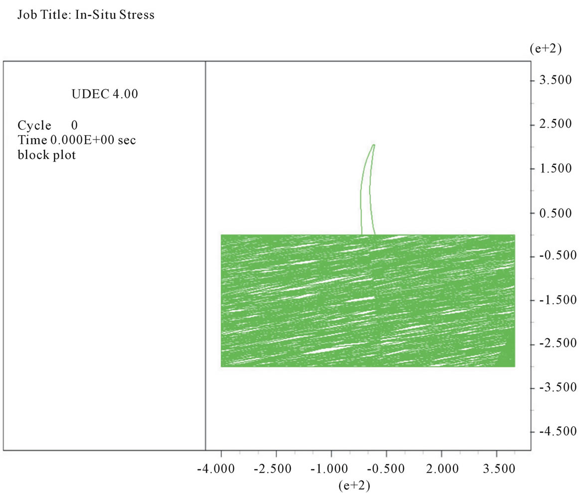
Figure 2. Structural model of dam and its foundation in the software.
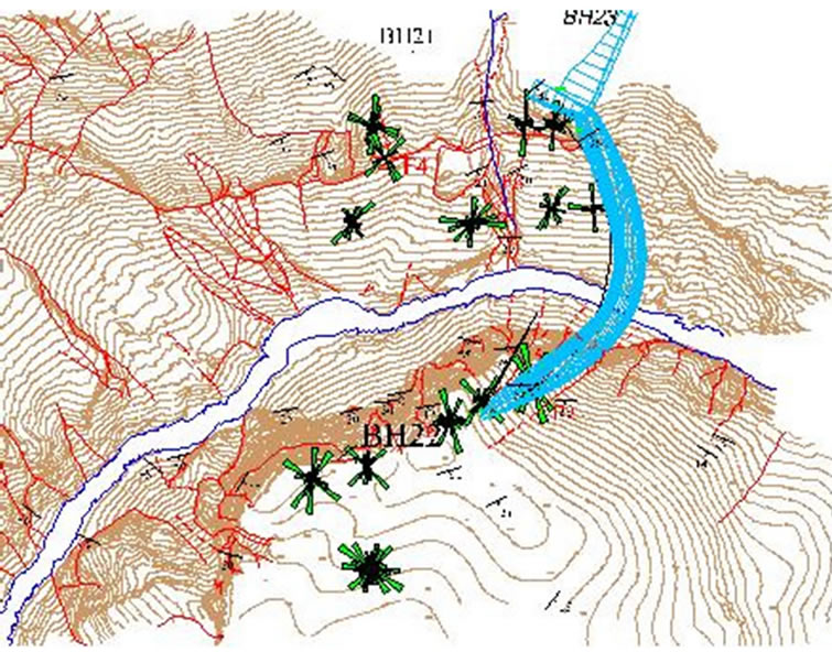
Figure 3. Joints and faults have affected the abutments of dam.
shallow depths or low confining stress levels, the compressibility of the intact rock makes a large contribution to the compressibility of a rock mass as a whole. Thus, the Poisson’s ratio of the intact rock has a significant effect on the Poisson’s ratio of a jointed rock mass.
The selection of properties is often the most difficult element in the generation of a model because of the high uncertainty in the property database. It should be kept in mind when performing an analysis, especially in geomechanics, problem will always involves a data limited system; the field data will never be known completely. However, with the appropriate selection of properties based upon the available database, important insight to the physical problem can still be achieved [1,3]. Now, the material behavior models are assigned for both blocks and discontinuities in the model.
2.3.1. The Behavioral Model of Intact Rock
The Mohr-Coulomb plasticity model is used for materials that yield when subjected to shear loading, but the yield stress depends on the major and minor principal stresses only; the intermediate principal stress has no effect on yield [2].
For the Mohr-Coulomb plasticity model in UDEC, the required properties are: density, Bulk modulus, shear modulus, friction angle, cohesion, dilation angle and tensile strength of rock mass. In UDEC, laboratory measured parameters shouldn’t directly be used in full scale. The existence of discontinuities reflects the real situation in the model but, some factors such as joints and tiny fractures should be considered in the rock mass [1,2].
Based on geological studies, dam foundation is made of dolomitic limestone, which its samples were used in three-axial compressive tests. According to this, first, by the help of results of compressive tests done on the digging core samples, it has been tried to estimate the
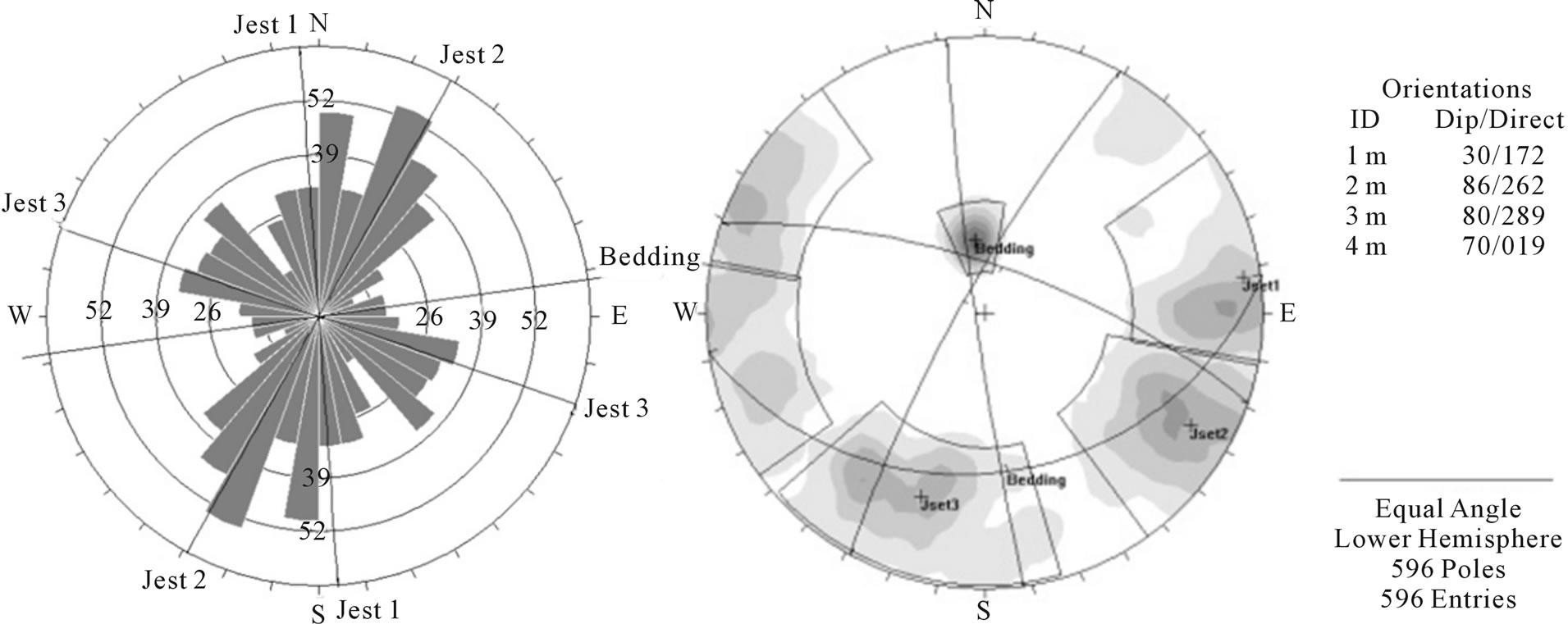
Figure 4. Discontinuities contour and its rose diagram which were applied in the software.
amounts of parameters of intact rock to some extent, then by the help of different classifications of rock mass such as Q, RMR, GSI and the failure criteria, the parameters of rock mass were estimated. The selected GSI for rock mass was 45 - 55, in spite of this matter that the resistance of rock mass is reduced after filling the reservoir with water, GSI = 50 was considered. On the other hand, the results of triaxial tests on saturated samples were used. The whole related processes were done by the Roclab software designed by Hoak. Thus the details of triaxial tests (σ1, σ3) on the selected samples were applied in Roclab software and (mi, σci, σcm) were gained. The results are listed in Table 1.
2.3.2. The Behavioral Model of Discontinuities
In addition to block material models, a constitutive model must also be assigned to all discontinuities in the model. The behavioral model of discontinuities shows the physical reaction of rock joints. The sufficient model for most analysis is the (elastic-perfectly plastic) coulomb slip model, which is assigned to discontinuities with the commands. This model is the most applicable model for the usual engineering studies, and the cohesion and friction angle which are needed in this model, often are more available than other joint properties. If coulomb slip model is used for simulating the discontinuities behavior, the following properties will be used: Friction angle of joint, cohesion of joint surface, dilation angle, tensile strength, normal stiffness and shear stiffness [1,2].
Joint properties are conventionally derived from laboratory testing (e.g., triaxial and direct shear tests). Joint resistance parameters; cohesion = 0.247 Mpa and friction angle of joint surface = 31º were estimated by the help of direct shear tests along the joints in the laboratory. Joints were almost without filling and occasionally stained with Ferro oxide. Values for normal and shear stiffnesses for rock joints typically can range from roughly 10 to 100 MPa/m for joints with soft clay in-filling to over 100 GPa/m for tight joints in granite and basalt. Published data on stiffness properties for rock joints are limited; summaries of data can be found in Kulhawy (1975), Rosso (1976), and Bandis et al. (1983).
Approximate stiffness values can be back-calculated from information on the deformability and joint structure in the jointed rock mass and the deformability of the intact rock. If the jointed rock mass is assumed to have the same deformational response as an equivalent elastic continuum, then relations can be derived between jointed rock properties and equivalent continuum properties.
For uniaxial loading of rock containing a single set of uniformly-spaced joints oriented normal to the direction of loading, the following relation applies [4]:
Kn = ErEm/s(Er − Em) (1)
where Em = rock mass Young’s modulusEr = intact rock Young’s modulusKn = joint normal stiffness, and s = joint spacing.
A similar expression can be derived for joint shear stiffness:
Ks = GrGm/s(Gr − Gm) (2)
where Gm = rock mass shear modulusGr = intact rock shear modulus, and ks = joint shear stiffness.
Several expressions have been derived for twoand three-dimensional characterizations and multiple joint sets. References for these derivations can be found in Singh (1973), Gerrard (1982), and Fossum (1985). It is important to recognize that joint properties measured in the laboratory typically are not representative of those for
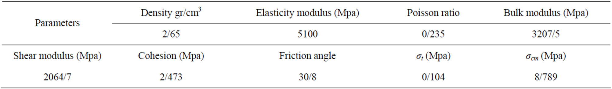
Table 1. The required properties of plasticity model of intact rock which are used in the software.
real joints in the field. Scale dependence of joint properties is a major question in rock mechanics.
Joint shear stiffness is the slope of the shear stressshear displacement curve until slip. For calculating the amounts of joints shear stiffness (ks), 5 direct shear tests done along the dolomitic limestone joints under different normal stresses, were selected. One of these direct shear tests which is used for calculating the amounts of KS is shown in Figure 5.
For this purpose, the slope of shear stress-displacement curves were obtained at different amounts of normal stresses, were used and ks of joints were calculated in each normal stress. Figure 6 shows the changes of ks versus the changes of normal stress in direct shear tests along the joints. Totally, the amounts of ks increase linear with the raise of normal stress on the joint. Then, conesquently ks increases with depth. Therefore, the amounts of ks of each joint sets in each depth were evaluated and implemented with special command in UDEC. By increasing the depth, shear stiffness rises so that in high level of stresses in high depth, shear stiffness reaches point that reflects the properties of intact rock.
There is another non-linear joint model in UDEC, which directly utilizes index properties from laboratory test results, which is Barton-Bandis joint model. A series of empirical relations has been developed by Drs. Nick Barton and Stavros Bandis to describe the effects of surface roughness on discontinuity deformation and strength. These relations, known collectively as the Barton-Bandis joint model, have been implemented into UDEC. This model is a non-linear joint model that directly utilizes index properties from laboratory test results relating joint shear stress to shear and normal displacement on joints. A complete explanation of these relations can be obtained from Barton (1982) and Bandis et al. (1985) [5]. Therefore, the index properties from laboratory test results, especially the effects of surface roughness on discontinuity deformation, are directly implemented in the software.
2.4. Boundary Conditions
The boundary conditions in a numerical model consist of the values of field variables e.g. stresses and displacements, which are prescribed at the boundary of the model before analysis. Boundaries are of two categories: real and artificial. Real boundaries exist in the physical object being modeled e.g. a tunnel surface or the ground surface. Artificial boundaries do not exist in reality, but they must be introduced in order to enclose the chosen number of elements (i.e. blocks). By default, the boundaries of a UDEC model are free of stress and any constraint. Forces or stresses may be applied to any boundary, or part of a boundary, by means of the commands [1].
2.5. In-Situ Stresses Conditions
In all civil or mining engineering, there is an in-situ state of stress in the ground before any excavation or construction is started. By setting initial conditions in the UDEC model, an attempt is made to reproduce this insitu state, because it can influence the subsequent behavior of the model. Ideally, information about the initial state comes from field measurements but when these are not available, the model can be run for a range of possible conditions.
In a uniform layer of soil or rock with a free surface, the vertical stresses are usually equal to ɡρz, where ɡ is the gravitational acceleration, ρ is the mass density of the material, and z is the depth below surface. However, the in-situ horizontal stresses are more difficult to estimate. There is a common belief that there is some natural ratio between horizontal and vertical stress, given by K = ν/1 − ν, where ν is the Poisson’s ratio. This formula is derived from the assumption that gravity is suddenly applied to an elastic mass of material in which lateral movement is prevented. This condition hardly ever applies in practice due to repeated tectonic movements, material failure, overburden removal and locked-in stresses due to faulting and localization [6].
The amounts of K by Hoak & Brown (1978) and Sheory (1994) equations are calculated for the valley of dam site and are applied averagely to the model in each depth. However, a set of stresses is installed in the model and then UDEC is run until an equilibrium state is obtained.
2.6. Loading and Fluid Flow Modeling
Following stage is loading and fluid flow modeling. The main purpose of this stage, is the simulating the different construction processes. The UDEC fluid flow logic is based on the assumption that blocks are impermeable.
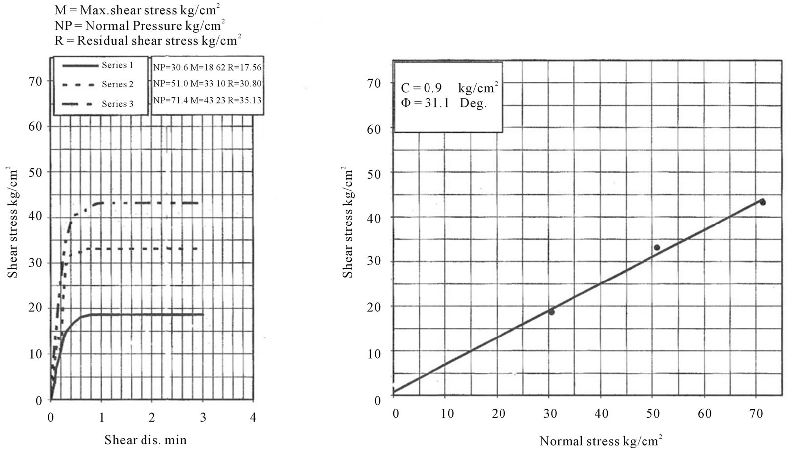
Figure 5. One of the direct shear tests which is used for calculating the amounts of joint shear stiffness.
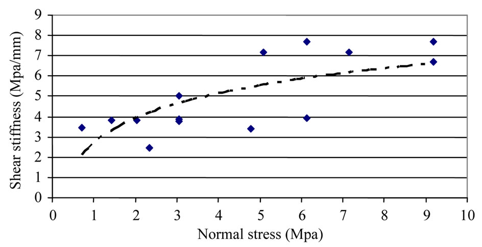
Figure 6. The changes of ks versus the changes of normal stress in shear tests which are done along the joints.
As a consequence of engineering works in a rock mass, deformation of both the joints and intact rock will usually occur as a result of stress changes. Due to the stiffer rock matrix, most deformation occurs in the joints, in the form of normal and shear displacement. If the joints are rough, deformations will also change the joint aperture and fluid flow.
In a rock mass, mechanical deformations will mainly occur as normal and/or shear deformations in the joints. This deformation will also change the joint aperture. By coupling the mechanical aperture changes to the hydraulic aperture changes, a hydro-mechanical coupling is achieved [1,7,8].
Fluid flow through a porous medium such as many soils and sedimentary rocks can be described by Darcy’s law (1-D flow):
Q = K·i·A (3)
where Q is the volumetric flow per unit area A, normal to the flow. Q is thus related to the dimensionless hydraulic gradient i, in the direction of the flow and to the hydraulic conductivity K. The latter is a material property of both the fluid and the geological medium and may be written as K = kρɡ/µ (4)
where k is the intrinsic permeability, ɡ is the acceleration due to gravity (9.81 m/s2), µ is the dynamic viscosity of the fluid (1 × 10⁻³ Ns/m2 for pure water at 20˚C) and ρ is the fluid density (998 kg/m3 for pure water at 20˚C).
For fluid flow through rock joints, it is common to consider the joint as composed of two smooth parallel plates and the flow to be steady, single phase, laminar and incompressible. Under these conditions, the hydraulic joint conductivity (Kj) may be written:
Kj = ρɡe2/12µ (5)
Kj = ɡe2/12ν (6)
where ν is the kinematic viscosity of the fluid (1 × 10⁻⁶ m2/s for pure water at 20˚C) and e is the hydraulic aperture. The hydraulic joint conductivity is a parameter expressing the flow through the joint under the influence of frictional losses, tortuosity and channel-ling; these factors depend on the geometry of the flow channels and the fluid viscosity. Assuming that Darcy’s law can also be applied to flow in rock joints, setting A = ew, we obtain Q = ɡwe3i/12ν (7)
where i is the dimensionless hydraulic gradient and w is the breadth of the flowing zone between the parallel plates. This equation is usually called the “cubic law”. One must keep in mind that Equation (7) is derived for an “open” channel, i.e. the planar surfaces remain parallel and are thus not in contact at any point.
Traditionally, fluid flow through rock joints has been described by the cubic law, which follows the assumption that the joints consist of two smooth, parallel plates. Real rock joints, however, have rough walls and variable aperture, as well as asperity areas where the two opposing surfaces of the joint walls are in contact with each other. Joint permeability is completely dependent on joint aperture (because of the third power of joint hydraulic aperture in cubic law). According to this, apertures can generally be defined as mechanical (E) and hydraulic (e) apertures.
The mechanical joint aperture (E) is defined as the average point-to-point distance between two rock joint surfaces. Often, a single, average value is used to define the aperture. The aperture distribution of a joint is only valid at a certain state of rock stress and pore pressure.
If the effective stress or the lateral position between the surfaces changes, as during shearing, the aperture distribution will also be changed. The hydraulic aperture (e) can be determined both from laboratory fluid flow experiments and bore-hole pump tests in the field. Due to the effects of roughness and tortuosity of flow, the fracture conductivity in Witherspoon (1980) experiments, was reduced by a factor between 1.04 and 1.65. Results by Hakami showed that the ratio between mechanical mean aperture (E) and hydraulic aperture (e) was 1.1 - 1.7 for joints with a mean aperture of 100 - 500 mm.
On the basis of experimental data, Barton et al. (1985) proposed an empirical formula that gives the hydraulic aperture (to be used in cubic law) as a function of the mechanical aperture and joint roughness coefficient (JRC).
e = E2/JRC2.5 (8)
One should note that this equation is only valid for E ≥ e. The JRC coefficient describes the peak roughness of correlated, mated surfaces, and can be estimated either by correctly designed tilt, push or pull tests on jointed rock samples or by visual comparison of measured roughness profiles from the joint surface with a standard set of profiles. The latter is obviously slightly objective, during shearing; this regular exponential behavior appears to break down. Under an increasing shear displacement the joint dilates and both the hydraulic and the mechanical aperture increase.
Then Olsson and Barton (2001) proposed an improved model on the basis of the performed hydro-mechanical shear tests. It is an empirical engineering model and not a theoretical scientific model. As shear tests on rough rock joints are composed of at least two major parts, pre peakpeak and post-peak, depends on shear displacement. The model considers these two basic phases. In the first phase, where the joint wall roughness is not destroyed, the peak JRC should be used in Equation (8) and hydraulic aperture (e) can be calculated by Equation (8) up to 0.75 peak shear displacement (δS ≤ 0.75δSP)
e = E2/JRC2.5 (8)
In the second phase, where the geometry of the joint walls is changing with increasing shear displacement, the JRCmob (mobilized value of JRC) should be used. Hydraulic aperture (e) can be calculated by Equation (9) for δS ≥ δSP (peak shear displacement)
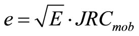 (9)
(9)
During this phase, gouge is being produced but as the joint is dilating, some of the gouge is probably flushed to the sides of developing flow channels. Based on normal loading/unloading, during increased normal stress, the hydraulic aperture (e) decreases, which causes an increase in E/e due to tortuosity. In shear behavior, during the first part of each plotted shear path in Figure 7, the E/e ratio is first slightly decreasing and thereafter increasing.
This initial part in this figure belongs to the pre peakpeak shear displacement. When the asperities along the joint walls are not destroyed and the hydraulic aperture is probably decreasing due to shear-related closing of small voids. Thereafter the geometry of the joint walls is in a changing phase (breakdown) where the asperities get worn and damaged under the increasing shear deformation. The size of roughnesses decrease in JRCmob depends
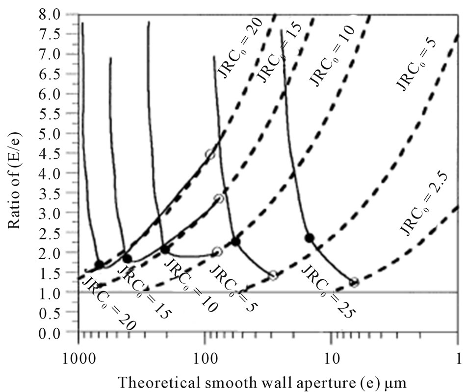
Figure 7. Curves relating the hydraulic aperture e and the ratio E = e for both normal and shear behavior.
on the strength of the asperities, on the applied normal load and on the shear deformation. Furthermore new flow paths open and others close due to the increasing areas of contact between the joint walls and due to gouge production. The gouge production will probably decrease the hydraulic aperture. So, the increase in E/e during shearing depends not on the same phenomena as during normal loading and unloading [8-10].
Figure 8 illustrates the changes of joints mechanical aperture versus the changes of normal stress in shear tests along the joints. As it’s illustrated in Figure 8, with increasing normal stress on the joints, the mechanical aperture of joints decreases. Consequently hydraulic aperture and finally joint permeability reduce too. Based on this, it’s concluded that with increasing depth, the apertures decrease and as a result, joint permeability reduces.
Hydro-mechanical shear tests have shown a widely used constitutive model that are included in the UDECBB code and yields results that are most suitable for normal loading and unloading and for shear with limited damage or gouge production.
So, for calculating conductivity changes of rock joints during shearing, one has first to assume the initial JRC value and the initial mechanical aperture. Thereafter, one has to calculate the changes of the mechanical aperture and JRCmob during shearing. These parameters should then be used in Equations (8) and (9) to calculate the changes of the hydraulic aperture during shearing. Therefore, it is possible to calculate the hydraulic conductivity of each joint set [8].
For this reason, the initial mechanical aperture of joints was measured 1 - 2 mm, Eo = 2 mm was selected and related calculations were done and the hydraulic conductivity of each joint set was evaluated. The results of calculating the mechanical and hydraulic apertures and hydraulic conductivity of each joint set are summarized in table 2.
Then, joint permeability factor, joint initial aperture in Zero normal stress and residual aperture must be defined based on particular commands for joint sets in software.
By setting the initial water table at free surface, the joint stresses will be calculated automatically to balance
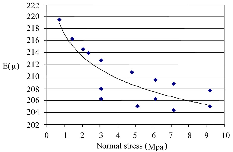
Figure 8. The changes of joints mechanical aperture versus the changes of normal stress in direct shear tests along the joints.
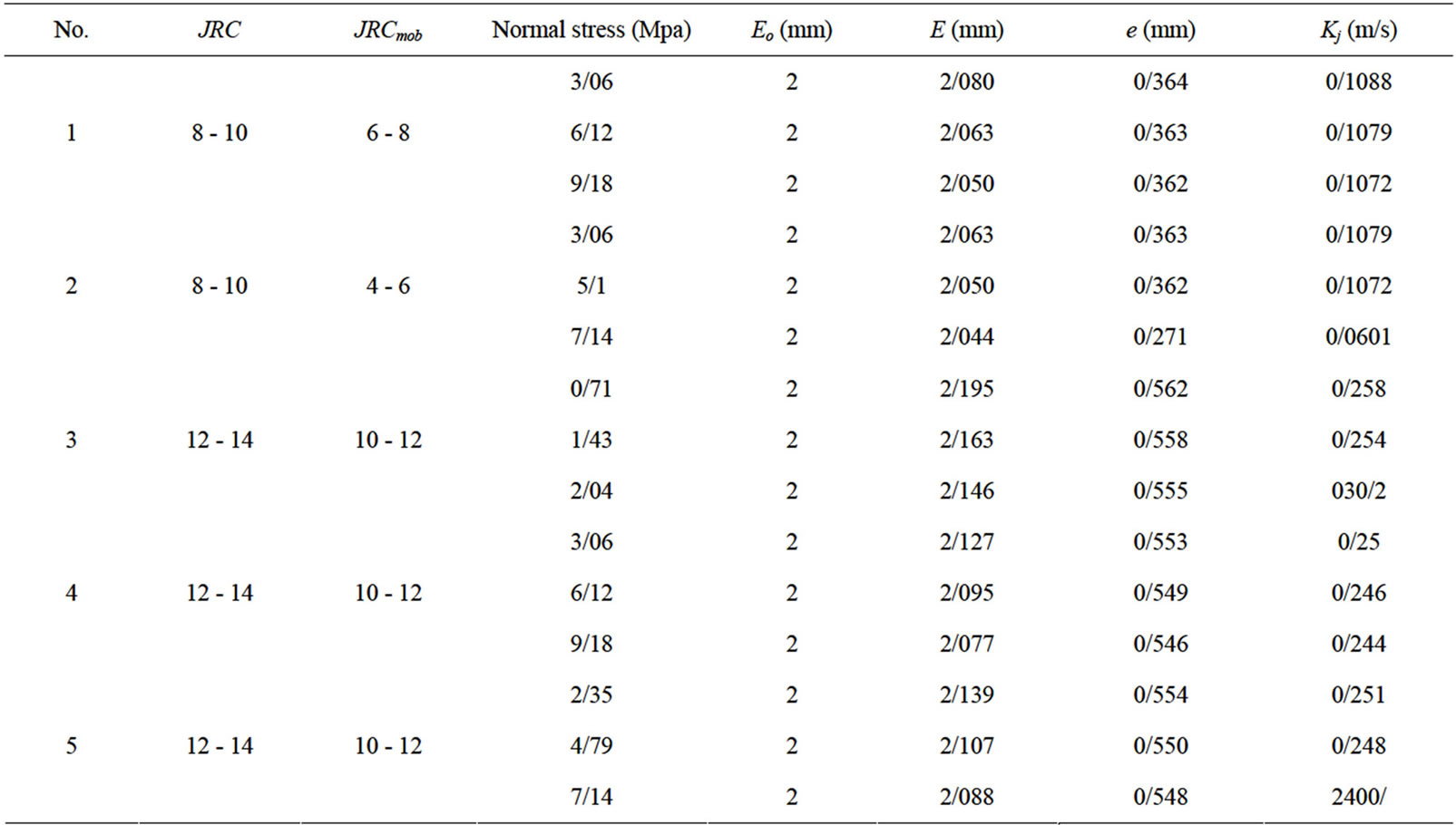
Table 2. The results of calculating the mechanical and hydraulic apertures and hydraulic conductivity of each joint set.
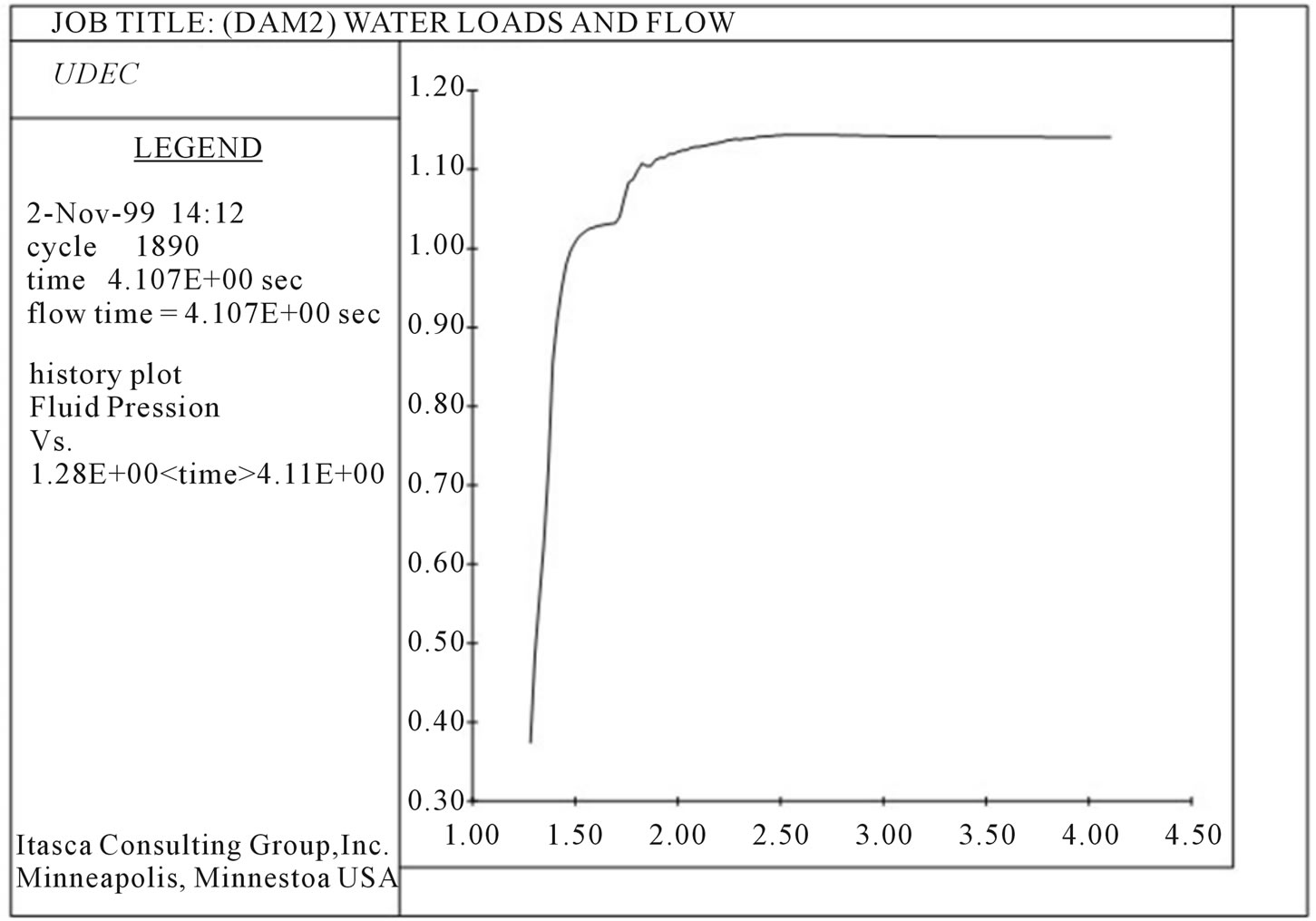
Figure 9. Fluid pressure in domain at location x, y.
the block stresses and domain pressures. The main flowrelated variables such as pressures and flow rates along a joint may be printed and plotted with special commands, and then numerical or graphical outputs are available. Histories of flow rates may be recorded at a particular contact or domain, too.
Therefore fluid flow from each point beneath the dam is separately accessible through drawn graphs by software. One of these graphs is shown in Figure 9.
With regarding in results of analysis, the seepage beneath the dam in full reservoir has a suitable situation and establishing a grout curtain with depth of 40 - 50 m seems to be adequate. Also, in abutments by considering the lower pressure of water, seepage reaches to a suitable condition in lower depths. In order to show the effect of the direction of joints on seepage, an impermeable curtain is modelized beneath the dam. The analysis results indicate the existence of inclined curtain, the seepage of dam foundation decreases more than when the curtain is vertical.
It should be considered that for estimating the depth of grouting curtain, some other parameters such as the topography, the lithology, reservoir level, groundwater situation, Lugeon and trial groutability results, boreholes arrangement and etc. must be noticed, too. But, however, a numerical analysis is useful for making a portrait from the mechanism which will be occurred.
3. Conclusion
UDEC has the capability to perform the analysis of fluid flow through the fractures of a system of impermeable blocks. A fully coupled mechanical-hydraulic analysis is performed, in which fracture conductivity is dependent on mechanical deformation and, conversely, joint water pressures affect the mechanical computations. By the help of Data’s obtained from numerical analysis, the seepage beneath dam foundation is estimated in full reservoir situation. With regarding in results of analysis, the seepage beneath the dam has a suitable situation and establishing a grout curtain with depth of 40 - 50 m seems to be adequate. Also, in abutments by considering the lower pressure of water, seepage reaches to a suitable condition in lower depths.
REFERENCES
- ITASCA Consulting Group Inc., “UDEC online Manual,” 2004. http://www.itascacg.com/udec/index.php
- P. Cundall, “A Generalized Distinct Element Program for Modeling Jointed Rock,” Report PCAR-1-80 US Army, Peter Cundall Associates, London, 1980.
- S. Bandis, “Engineering Properties and Characterization of Rock Discontinuities,” In: S. Bandis, Ed., Comprehensive Rock Engineering: Principles, Practice & Projects, Pergamon Press, Oxford, 1993, pp. 18-155.
- R. E. Goodman, “Introduction to Rock Mechanics,” 2nd Edition, John Wiley & Sons Ltd., Hoboken, 1989.
- S. D. Priest, “Discontinuity Analysis for Rock Engineering,” Chapman & Hall Press, London, 1993. doi:10.1007/978-94-011-1498-1
- E. Hoek and E. T. Brown, “Practical Estimation of Rock Mass Strength,” International Journal of Rock Mechanics & Mining Sciences, Vol. 34, No. 8, 1997, pp. 1165-1186. doi:10.1016/S1365-1609(97)80069-X
- N. Barton, S. Bandis and K. Bakhtar, “Strength Deformation and Conductivity Coupling of Rock Joints,” International Journal of Rock Mechanics & Mining Sciences, Vol. 22, No. 3, 1985, pp. 40-121.
- R. Olsson and N. Barton, “An Improved Model for Hydro- Mechanical Coupling during Shearing of Rock Joints,” International Journal of Rock Mechanics & Mining Sciences, Vol. 38, No. 3, 2001, pp. 317-329. doi:10.1016/S1365-1609(00)00079-4
- R. Olsson, “Mechanical and Hydro-Mechanical Behavior of Hard Rock Joints—A Laboratory Study,” Ph.D. Thesis, Chalmers University of Technology, Gothenburg, 1998.
- R. Olsson, “Mechanical and Hydro-Mechanical Behavior of Hard Rock Joints—A Laboratory Study,” Addendum Report 6, Chalmers University of Technology, Gothenburg, 1999.