Current Urban Studies
Vol.06 No.04(2018), Article ID:88966,18 pages
10.4236/cus.2018.64027
Measuring Urban Sprawl Indices at Traffic Analysis Zone (TAZ) Level
Tahmina Khan, Michael Anderson
Department of Civil and Environmental Engineering, The University of Alabama in Huntsville, Huntsville, AL, USA

Copyright © 2018 by authors and Scientific Research Publishing Inc.
This work is licensed under the Creative Commons Attribution International License (CC BY 4.0).
http://creativecommons.org/licenses/by/4.0/


Received: August 27, 2018; Accepted: December 2, 2018; Published: December 5, 2018
ABSTRACT
High rates of land use change causing unsustainable development have attracted the attention of policy and planning and raised the need to understand the factors behind it. Sprawl occurs because of the residents’ preference to live in suburbs, low-cost auto travel, technological innovations, the aspiration for urbanized-automobile dependent lifestyle, the disappearance of rural agricultural land, and spatial fragmentation. Thus, it induces sustainability challenges and leads to excessive commuting and congestion. There is a greater necessity to quantify urban sprawl at Traffic Analysis Zone level so that transportation and land use planners can identify potential sprawling TAZ and can promote/develop sustainable strategies for future land use planning. In this study, sprawling indices at TAZ level were derived with and without incorporating centering effect and compared the scores of sprawling TAZs in 2010 to the sprawling TAZs for 2000. The main goal was to propose a methodology for determining potential sprawling TAZs and to identify locations responsible for sprawl in a case study city. The results can be a substantial input in planning and decision-making process.
Keywords:
Sustainability, Urban Sprawl Indices, Principal Components, Potential Sprawling Traffic Analysis Zone

1. Introduction
Landscapes are dynamic, and change is one of their properties where humans have always adapted their environment to better fit the needs and thus reshaped the landscape. All the important driving forces towards the societal change are related to the population growth and the lifestyle is becoming increasingly urban and more mobile. The analysis of the nature and causes of landscape changes in the past centuries show three main driving forces, such as accessibility, urbanization, and globalization that affected the nature and pace of the changes as well as the perception people have had about the landscape (Antrop, 2005) . During the last decades, high rates of change causing unsustainable development have attracted the attention of policy and planning and raised the need to understand the factors behind it. The road network shows a continuous growth and the built-up area shows a continuous expansion, both corresponding to positive transformation rates that mean both contribute an increase in respective landscape elements (Schneebergera et al., 2007) . Driven apart, a new report from CEOs for Cities unveils the real reason Americans spend so much time in traffic because of sprawl which is the real cause of traffic congestion and the solution to this problem has much more to do with how we build our cities than how we build our roads (Cortright, 2011) . Sprawl means low density, sometimes dispersed, sometimes decentralized, sometimes polycentric, sometimes suburban development (strip, scattered, and leapfrog developments), caused by the consumer preference to live in suburbs, low-cost auto travel, technological innovations, subsidies and public and quasi-public goods (Ewing, 1997) . It is often difficult to distinguish these development patterns. One sprawl indicator is the land use density function, and Ewing definition of sprawl is shown graphically in Figure 1(a) where few significant centers, low average density, and noticeable development gaps exist due to leapfrogging, which all impose high and avoidable infrastructure, travel, energy, and environmental costs (Zhang, 2010) .

Figure 1. Definition of sprawl and decentralization (Zhang, 2010) . (a) Sprawl; (b) Polycentric efficient pattern.
Therefore, sprawl induces higher than the necessary total social costs in terms of poor accessibility, excessive commuting, infrastructure supply, environmental damages, and other externalities. Figure 1(b) shows a potentially efficient urban form, a polycentric pattern with moderate densities and continuous land use except for permanent open spaces. Figure 1(c) illustrates a compact monocentric pattern, which will be referred to as a centralized pattern. Any land use change causing employment or housing density distributions to differ from this centralized pattern will be referred to as decentralization. Apparently, decentralization does not necessarily imply sprawl (Zhang, 2010) . In contrast to sprawl, compactness can preserve agricultural land, promote high capacity transit systems and helps to lower automobile dependency for households, reduce environmental destruction and prevent moral minimalism (Gordon & Richardson, 1997) .
Economists believe that three underlying forces―population growth, rising household incomes (demand more living space), and transportation improvements―are responsible for this spatial growth and urban sprawl. Moreover, three market failures such as failure to take into account the social value of open space, failure to recognize the social costs of congestion, and failure of real estate developers to take into account all of the new development costs are the main causes of urban sprawl. The three remedies, namely, development taxes, congestion tolls, and impact fees were prescribed for the market failures leading to urban sprawl where each involves the use of the price mechanism. For instance, development taxes on each acre of land converted from agricultural to urban use, raising commuting costs by imposing a congestion toll and correcting impact fees for new developments are suggested remedies (Brueckner, 2000) . A paper “The Effects of Urban Sprawl on Daily Life” mentioned about a project that analyzed the use of transit-oriented development (TOD) in conjunction with a light rail system as an alternative to a proposed highway bypass. This paper concluded that the light rail/TOD strategy could significantly reduce congestion, automobile trips, VMT, and air pollution emissions over the highway bypass alternative. It shows the Atlantic Steel (Atlantic Station) Smart Growth project does prove to be a valuable strategy to lessen some of the effects of urban sprawl, mostly VMT; however, it is costly to implement (Brunner, 2013) .
It can be understood that sprawl is happening because of the population growth, the aspiration for urbanized-automobile dependent lifestyle, the disappearance of rural agricultural land, and spatial fragmentation. Thus, it induces sustainability challenges (Luoa & Dennis Wei, 2009) and causes to excessive commuting and congestion. There is a greater necessity to quantify urban sprawl at Traffic Analysis Zone level so that transportation and land use planners can identify potential sprawling TAZ and can promote/develop sustainable strategies in an efficient and creative manner.
Huntsville is the fastest growing major metro area in the state of Alabama, accounted for 34% of Alabama’s Growth in population, and employment growth exceeds Alabama as a whole. The community and local business owners continue to be very positive, and the trend toward new growth is certain (Huntsville, 2015) . The spatial configuration of new developments in Huntsville has already reflected a prominent scattered, and leapfrog pattern. An inevitable consequence of growing trend of sprawl includes the growth outwards of the city and its suburbs to its outskirts to low-density, and auto-dependent development on rural land. There is no doubt that the demand for urban land and the pressure for sustainable development will increase in Huntsville near future. Better understanding and managing of urban growth are critical to the development and sustainability in any city. Because of the availability of the recent methodology on measuring sprawl for larger areas (Ewing & Hamidi, 2014) , relevant data and advanced tools to process and analyze data, it has been vital and attainable to measure sprawl at TAZ level. It can address sustainability and a proper balance between the extents of compactness and sprawling can be established at TAZ level for future land use planning.
In this study, sprawling indices at TAZ level were derived with and without incorporating centering effect and compared the scores of sprawling TAZs in 2010 to the sprawling TAZs for 2000. The main goal was to propose a methodology for determining potential sprawling TAZs for Huntsville. This study can help to demonstrate the locations responsible for sprawl in Huntsville. The results can be a substantial input in planning and decision-making process.
2. Recent Studies on Measuring Urban Sprawl
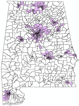
The original sprawl indices were available to researchers and have been widely used in outcome-related research since sprawl has been linked to physical inactivity, obesity, traffic fatalities, poor air quality, residential energy use, emergency response times, teenage driving, lack of social capital, and private-vehicle commute distances and times. Refined versions of the indices defined/shown in “Measuring Sprawl 2014” capture four distinct dimensions of sprawl for instance development density, land use mix, population and employment centering, and street accessibility. Compactness indices/sprawl-like metrics for census tracts within metropolitan areas were derived through the use of variables applied in larger area analyzes (metropolitan area, urbanized area, and county sprawl metrics). Principal components were extracted from multiple variables using principal component analysis and transformed the first principal component to an index with the mean of 100 and a standard deviation of 25. Figure 2(a) and Figure 2(b) present census tracts (Purple and Green) for Alabama and Huntsville respectively that were included to estimate sprawl metrics in “Measuring Sprawl 2014” (Ewing & Hamidi, 2014; National Cancer Institute, n.d.) .
It can be mentioned that a study on quantifying sprawl index used the methodology for generating a sprawl index for Metropolitan Statistical Areas (MSAs) developed by Reid Ewing (Jessup, 2014) . Likewise, this study implemented the methodology applied for measuring a sprawl index for census tracts.
(a)
 (b)
(b)
Figure 2. Metrics for census tracts (a) Alabama and (b) Huntsville (National Cancer Institute, n.d.) .
3. Case Study
The Huntsville, Alabama Metropolitan Planning Area (MPA) includes all of Madison County and part of Limestone County shown in the following snapshot from Google Earth with well-defined Traffic Analysis Zones (TAZs). The metro area is around 947 square miles and has a population of 363,210 people with 156,649 households (United States Census Bureau, 2010) . Population and household data are available as statewide block level shapefile for 2010 (United States Census Bureau, 2010) and summarized in ArcGIS to know the required values at MPA level. There are 525 Traffic Analysis Zones in the network of which 508 are internal zones, and 17 are external zones (Figure 3).
Following sections contain several key parts to explain the variables, analysis, and results, validation, and findings.
4. Data Collection and Analysis
Compactness indices/sprawl-like metrics for census tracts within metropolitan areas were derived through the use of following variables (shown in Table 1). Table 2 demonstrates the corresponding equation to determine variables at TAZ level where census block was used to achieve our desired resolution.

Table 1. TAZ sprawl index variables.
Table 2. Equations to compute variables associated with sprawl.

Figure 3. Study area.
Employment data are accessible from the Local Employment Dynamics (LED) database that is assembled by the Census Bureau through a voluntary partnership with state labor market information agencies (Ewing & Hamidi, 2014) . Workplace Area Characteristic data are collected at census block geography level and can be aggregated to any larger geography, in this case, Traffic Analysis Zone when it is required. LED data were processed for the year 2002 and 2010 that included a total number of jobs and the number of employment by two-digit NAICS (North American Industry Classification System) code. The data were aggregated to generate total jobs by one-digit NAICS code for every block under any particular TAZ.
Because of unavailability of Walk Score related data, a new variable was introduced to measure the walkability. From any grocery shop to a TAZ block, if the nearest distance is within 1.5 miles, those values were inversed and weighted by the sum of block level population and employment as a percentage of the TAZ total to obtain Grocery/Amenity reachability index.
Where, i is the census block number, n is the number of blocks in the TAZ, Ji or BJi is jobs in census block, Pi or BPi is residents in census block, JP is jobs per person in the metropolitan area, TJ is the total jobs in the TAZ, Pj is proportion of jobs in sector j, and j is the number of sectors.
Population, employment, block and road shapefiles were gathered for the year 2000 and 2010 and processed to calculate the above variables according to the equations mentioned in Table 2. Principal component analysis (PCA) was executed for both 2000 and 2010. However, road shapefile of 2000 was used in both cases as 2010 road shapefile provides too many segments without being merged into one single centerline and it does not supply the endpoints either as start or end node. Principal components were extracted from multiple variables using principal component analysis and transformed the first three principal components to an index with the mean of 100 and a standard deviation of 25. For the sake of consistency and ease of understanding, this transformation was conducted. The more compact counties have index values above 100, while the more sprawling counties have values below 100. PCA was performed using Minitab® Statistical Analysis Software, Release 17 for each case (shown in Table 3) (Minitab Inc., 2015) . To introduce the centering effect, a new variable was added in our analysis. A centering factor was included to compare the results of PCA and to know how this can change the distribution for the entire study area. The following cases were built to compare indices with or without centering effect in our analysis.
5. Results
Principal component analysis was run to reduce above variables to a single index for each case. First, three principal components were summed so that the index can account for minimum 50 percent of the variance in the original variables. Table 4 presents the summation of first three eigenvalues and total variance by scenario.
Composite or compactness scores for the year 2000 and 2010 are presented in Figure 4 while analyzing data without the centering effect. It is apparent from Figure 4 that dispersed growth and compactness both change over a 10-year period. However, appropriate roadway data could have presented a little different spatial pattern while analyzing the year 2010. To determine how much land use pattern was changed from 2000 to 2010, the difference in sprawl indices was
Table 3. Building different cases.
Table 4. Eigenvalue and cumulative variance.
 (a)
(a) (b)
(b)
Figure 4. Compactness indices (a) Case 1a_00 and (b) Case 2a_10.
summed after assigning 100 for compact TAZs, which are equal to or greater than 100. Replacing value greater or equal to 100 can separate sprawling areas from compact ones. After that, subtracting 2000 indices from that of 2010 followed by the summation of the differences can provide an overall picture of sprawl for our study area. This value is +928; that means sprawling areas in 2000 are likely to continue its identical nature.
Figure 5 shows the spatial distribution of compactness indices that contains the centering factor as the inverse of distances from major city centers to TAZs. In scattered or leapfrog development, residents and service providers must pass by vacant land and in classic strip development, the consumer must pass other uses on the way from one store to the next. Thus, sprawl is associated with sparse street networks as well as dispersed land use patterns leaving residents with no alternative to long distance trips by automobile (Ewing & Hamidi, 2014) . In order to curtail scattered or leapfrog development, commercial strip development, uniform low-density development, or single-use development, this variable was introduced. This centering factor can redistribute the spatial pattern of sprawl indices (shown in Figure 5) such that TAZs far from city centers can be defined as scattered or leapfrog development. This way compact development can be centralized in which related land uses are highly accessible to one another, thus minimizing automobile travel and attendant social, economic, and environmental costs (Ewing & Hamidi, 2014) .
6. Validation
The recent report on urban sprawl (Ewing & Hamidi, 2014) validated their findings by inspecting Google Earth satellite images. About five most sprawling and compact TAZs determined by 2010 scores according to the variables were included in Figure 6 and Figure 7 that show Google Earth satellite images bounded by TAZs. Most of the sprawling TAZs in both sets of Figure 6 and Figure 7 have similar patterns of low-density development. And, compact TAZs in both cases (with or without centering factor) are a good representative of densely land use pattern.
It can be noted that TAZs with a higher value of Mahalanobis distance (Minitab Inc., 2015) cannot be a good representative for the study area and were excluded when the scores were sorted to rank those as the most compact or most sprawling TAZs.
Another initiative to compare 2010 results with the earlier findings (Ewing & Hamidi, 2014; National Cancer Institute, n.d.)
Figure 5. Compactness indices (a) Case 1b_00 and (b) Case 2b_10.
Figure 6. Most sprawling TAZs 1(a) through 1(e) and Most compact TAZs 2(a) through 2(e) (Case 2a_10).
Figure 7. Most sprawling TAZs 3(a) through 3(e) and Most compact TAZs 4(a) through 4(e) (Case 2b_10).
these average values are not comparable to the Tract Sprawl Indices, Figure 8 shows the variation of low and high that is quite analogous.
7. Findings
It is ostensibly from Figures 6-8 that sprawling/compactness indices coincide with the earlier conclusions and spatial patterns of satellite images. In this study, it is required to identify potential TAZs that can contribute sprawl. Both results from Case 2a_10 and Case 2b_10 were partitioned where sprawl indices are below 100. The number of TAZs (<100) equated in both cases is 214 which is very high comparing to the total number of TAZs. A threshold depending on the quartiles can be considered to lower the number of sprawling TAZs. For example, based on the maximum value of 75 percentiles of two cases (Case 2a_10 and Case 2b_10) that is about 92, TAZs were abstracted. TAZs were further filtered and separated if those are present in both cases. Hence, this screening process combines the outputs into one subset of TAZs. Table 5 provides the number of sprawling TAZs and its threshold.
Figure 9 shows the locations of 147 sprawling TAZs on a map view when the threshold is equivalent to 75 Percentile.
Figure 10 and Figure 11 present the locations of sprawling TAZs for 50 and 25 Percentiles respectively. These TAZs were examined in Google Earth and found to resemble the features of sprawling.
8. Conclusion
This study uses the recent methodology developed by Ewing and illustrates how the principal component analysis was used to derive compactness/sprawl indices at TAZ level. It provides a scoring system that analyzed available data with or without adding the centering variable for the year 2000 and 2010. The resulting compactness index conforms to the definition of sprawl in satellite imagery where development patterns are a good representative of sprawl.
The uniqueness of this paper is the inclusion and testing of centering factor which redistributes the spatial pattern of sprawl indices in such a way that TAZs far from city centers can be defined as scattered or leapfrog development. Another key finding is to identify potential TAZs contributing sprawl according to a threshold that combines both results (with or without centering effect).
The outcomes can be a substantial input in planning and decision-making process. Any preferred planning scenario can be tested for the betterment of sustainable transportation system where sprawling TAZs can be restricted to generate or attract any trips.
Table 5. Number of sprawling TAZs and its threshold.
 (a)
(a) (b)
(b)
Figure 8. Census Tract compactness index (a) Earlier results (National Cancer Institute, n.d.) (b) Summarized results.

Figure 9. Sprawling TAZs - 75 Percentile.

Figure 10. Sprawling TAZs - 50 Percentile.

Figure 11. Sprawling TAZs - 25 percentile.
Conflicts of Interest
The authors declare no conflicts of interest regarding the publication of this paper.
References
- 1. Antrop, M. (2005). Why Landscapes of the Past Are Important for the Future. Landscape and Urban Planning, 70, 21-34. https://doi.org/10.1016/j.landurbplan.2003.10.002 [Paper reference 1]
- 2. Brueckner, J. K. (2000). Urban Sprawl: Diagnosis and Remedies. International Regional Science Review, 23, 160-171. https://doi.org/10.1177/016001700761012710 [Paper reference 1]
- 3. Brunner, A. (2013). The Effects of Urban Sprawl on Daily Life: Smart Growth Implementation of Atlantic Station. Transportation Research Board. [Paper reference 1]
- 4. Cortright, J. (2011). CEOs for Cities. https://visual.ly/community/infographic/transportation/sprawl-crawl [Paper reference 1]
- 5. ESRI Data & Map. (2004). ArcGIS 9 Media Kit. Redlands, CA: ESRI. [Paper reference 4]
- 6. Ewing, R. (1997). Is Los Angeles-Style Sprawl Desirable?. Journal of the American Planning Association, 63, 107-126. https://doi.org/10.1080/01944369708975728 [Paper reference 1]
- 7. Ewing, R., & Hamidi, S. (2014). Measuring Urban Sprawl and Validating Sprawl Measures. Salt Lake City, Utah: Metropolitan Research Center. [Paper reference 7]
- 8. Gordon, P., & Richardson, H. W. (1997). Are Compact Cities a Desirable Planning Goal? Journal of the American Planning Association, 63, 95-106. https://doi.org/10.1080/01944369708975727 [Paper reference 1]
- 9. Huntsville, C. O. (2015). 2015 State of the Economy. Chamber of Commerce of Huntsville/Madison County. [Paper reference 1]
- 10. Jessup, J. (2014). Sprawl and Transportation Outcomes in Chicago: A Sprawl Index for Municipal Subsections. Transportation Research Board. [Paper reference 1]
- 11. Local Employment Dynamics. n.d. Longitudinal Employer-Household Dynamics. http://lehd.ces.census.gov/data/ [Paper reference 3]
- 12. Luoa, J., & Dennis Wei, Y. (2009). Modeling Spatial Variations of Urban Growth Patterns in Chinese Cities: The Case of Nanjing. Landscape and Urban Planning, 91, 51-64. https://doi.org/10.1016/j.landurbplan.2008.11.010 [Paper reference 1]
- 13. Minitab Inc. (2015). Minitab Statistical Software, Release 17. Pennsylvania: State College. [Paper reference 2]
- 14. National Cancer Institute. n.d. Updated Urban Sprawl Data for the United States. http://gis.cancer.gov/tools/urban-sprawl/ [Paper reference 42]
- 15. Schneebergera, N., Bürgi, M., Herspergerb, A. M., & Ewaldc, K. (2007). Driving Forces and Rates of Landscape Change as a Promising Combination for Landscape Change Research—An Application on the Northern Fringe of the Swiss Alps. Land Use Policy, 24, 349-361. [Paper reference 1]
- 16. United States Census Bureau. (2010). Tiger/Line Shapefiles. https://www.census.gov/geo/maps-data/data/tiger-line.html [Paper reference 9]
- 17. Zhang, L. (2010). Does Freeway Traffic Management Strategies Exacerbate Urban Sprawl: The Case of Ramp Metering. Transportation Research Board. [Paper reference 3]