Geomaterials
Vol. 2 No. 4 (2012) , Article ID: 24015 , 4 pages DOI:10.4236/gm.2012.24013
Geothermal Investigations in Permafrost Regions— The Duration of Temperature Monitoring after Wellbores Shut-In
1Pajarito Enterprises, Santa Fe, New Mexico, USA
2Department of Geophysics and Planetary Sciences, Raymond and Beverly Sackler Faculty of Exact Sciences, Tel Aviv University, Ramat Aviv, Tel Aviv, Israel
Email: levap@post.tau.ac.il
Received August 4, 2012; revised September 26, 2012; accepted October 7, 2012
Keywords: Permafrost; Formation Temperature; Shut-In Temperature; Deep Wells; Geothermal
ABSTRACT
The most important data on the thermal regime of the Earth’s interior come from temperature measurements in deep boreholes. The drilling process greatly alters the temperature field of formations surrounding the wellbore. In permafrost regions, due to thawing of the formation surrounding the wellbore during drilling, representative data can be obtained only by repeated observations over a long period of time (up to 10 years). Usually a number of temperature logs (3 - 10) are taken after the well’s shut-in. Significant expenses (manpower, transportation) are required to monitor the temperature regime of deep wells. In this paper we show that in most of the cases (when the time of refreezing formations is less than the shut-in time) two temperature logs are sufficient to predict formations temperatures during shut-in, to determine the geothermal gradients, and to evaluate the thickness of the permafrost zone. Thus the cost of monitoring the temperature regime of deep wells after shut-in can be drastically reduced. A simple method to process field data (for the well sections below and above the permafrost base) is presented. Temperature logs conducted in two wells were used to demonstrate utilization of this method.
1. Introduction
Temperature logs are commonly used to determine the permafrost temperature and thickness. When wells are drilled through permafrost, the natural temperature field of the formations (in the vicinity of the borehole) is disturbed and the frozen rocks thaw for some distances from the borehole axis. To determine the static temperature of the formation and permafrost thickness, one must wait for some period after completion of drilling before making geothermal measurements. This is socalled restoration time, after which the difference between the temperature of the formation and that of the fluid is less than the needed measurement accuracy. The presence of permafrost has a marked effect on the time required for the near-well-bore formations to recover their static temperatures. The duration of the refreezing of the layer thawed during drilling is very dependent on the natural temperature of formation; therefore, the rocks at the bottom of the permafrost refreeze very slowly. A lengthy restoration period of up to ten years or more is required to determine the temperature and thickness of permafrost with sufficient accuracy [1-6].
Earlier we suggested a “two point method” [7] which permits one to determine the permafrost thickness from short term (in comparison with the time required for temperature restoration) downhole temperature logs. The “two point method” of predicting the permafrost thickness is based on determining the geothermal gradient in a uniform layer below the permafrost zone. Only temperature measurements for two depths are needed to determine the geothermal gradient. The position of the permafrost base is predicted by the extrapolation of the static formation temperature-depth curve to 0˚C. It should be noted that here the permafrost base is defined as the 0˚C isotherm. Precise temperature measurements [2,3] taken in 15 deep wells located in Northern Canada (Arctic Islands and Mackenzie Delta) were used to verify the proposed method. Let us assume that at the moment of time t = tep the phase transitions (water-ice) in formations at a selected depth are completed, i.e. the thermally disturbed formation has frozen. In this case at t > tep the cooling process is similar to that of temperature recovery in sections of the well below the permafrost base. It is well known [8] that the freezing of the wateroc curs in some temperature interval below 0˚C (Figure 1). In practice, however, the moment of time t = tep cannot be determined. Only conducting long-term repetitive temperature observations in deep wells can do this. Earlier we assumed that three shut-in temperatures Ts1, Ts2, and Ts3 are measured at a given depth (Figure 1). For this case we proposed a method of predicting the formation temperatures [9].
A generalized formula to process field data (for the well sections below and above the permafrost base) was developed. Temperature logs conducted in five wells were used to apply this method [9].
It is demonstrated, by using field examples, that for deep boreholes several methods of predicting the permafrost temperature and its thickness should be applied. Low temperatures (from –15˚C to –5˚C) are typical for upper sections of the well’s lithological profile. In this case the refreezing period is short and the empirical formula [10] can be utilized to determine permafrost temperature and geothermal gradient) This is not the case for the lower sections of the wellbore where the surrounding formations are at high temperatures (from –3˚C to –1˚C). Here freezing time is large and only “three point” method is used.
The objective of this paper is to show that in many cases (when the time of refreezing formations is less than the shut-in time) two temperature logs are sufficient to predict formations temperatures during shut-in, to determine the geothermal gradients, and to evaluate the thickness of the permafrost zone.
2. Shut-In Temperatures—Permafrost Zone
In 1959 in their classical paper Lachenbruch and Brewer [10] proposed an empirical formula (Equation (1)) to predict the wellbore temperatures during shut-in.

Figure 1. Shut-in temperatures at a given depth (above the permafrost base)-schematic curve.
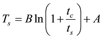 (1)
(1)
where A and B are empirical coefficients determined from field measurements.
It is a reasonable assumption that the value of tc (the “disturbance” period) is a linear function of the depth (h):
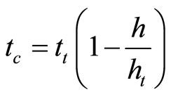 (2)
(2)
Equation (1) was successfully utilized to describe the measured shut-in temperature in the Well 3, Alaska, South Barrow. The well was drilled for 63 days to a total depth of 2900 ft. Temperature measurements to a depth of 595 feet were made during a period of six years after drilling. For the depth of 595 ft the average value of Tf is 6.568˚C (9 temperature logs). The completion of freezing occurred at temperature of about –0.6˚C and duration of the complete freezeback is approximately 20 days (Figure 2).
US Geological Survey conducted extensive temperature measurements in Alaska (US Geological Survey “Site” File-Alaska, Internet [11]). We selected long term temperature surveys in three wells (Table 1) to find out if the proposed Equation (6) (see Section 3) can be used when only two temperature logs are available. In Table 2 the calculated values of A and B for two wells are presented. For the well Drew Point No.1 we used the values of Ts measured in the first two temperature logs (ts1 = 186 days ts2 = 547days) to determine empirical coefficients A and B. After this we calculated values of Ts for the last temperature log (ts = 2339 days).
Similarly, for the well East Simpson #1 we used the values of Ts measured in the first two temperature logs (ts1 = 155 days, ts2 = 520 days) to obtain values of A and B. Values of Ts determined for ts = 1947 days (the last temperature log) are also presented in Table 2. From For mula 1 follows that at 
 . Assuming
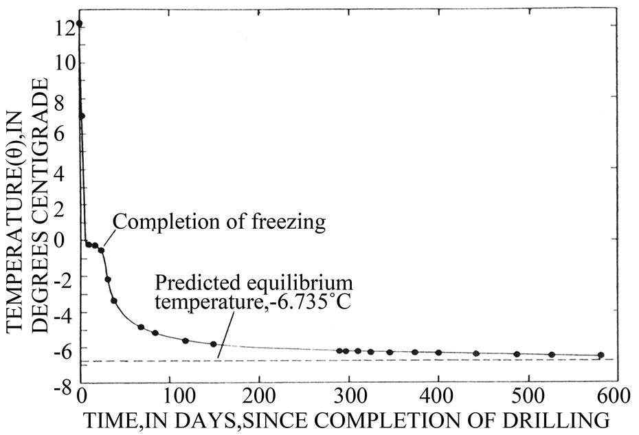
Figure 2. Cooling of South Barrow (Alaska) Well 3595-foot depth curve (after [10]).
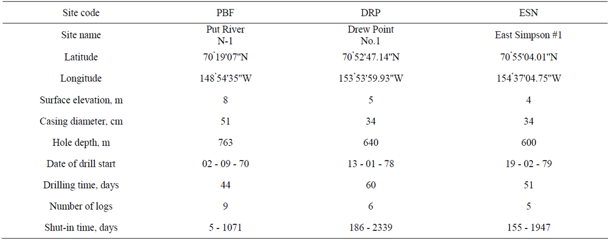
Table 1. Input data and location of three wells, Alaska, (US Geological Survey “Site” File-Alaska, Internet).
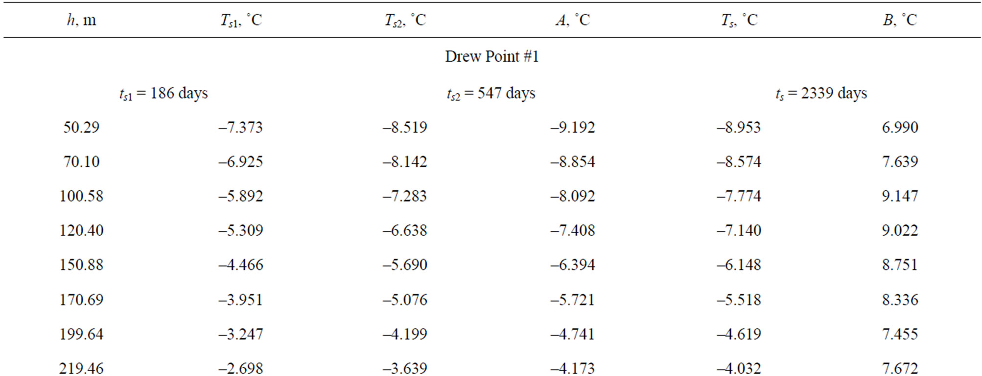
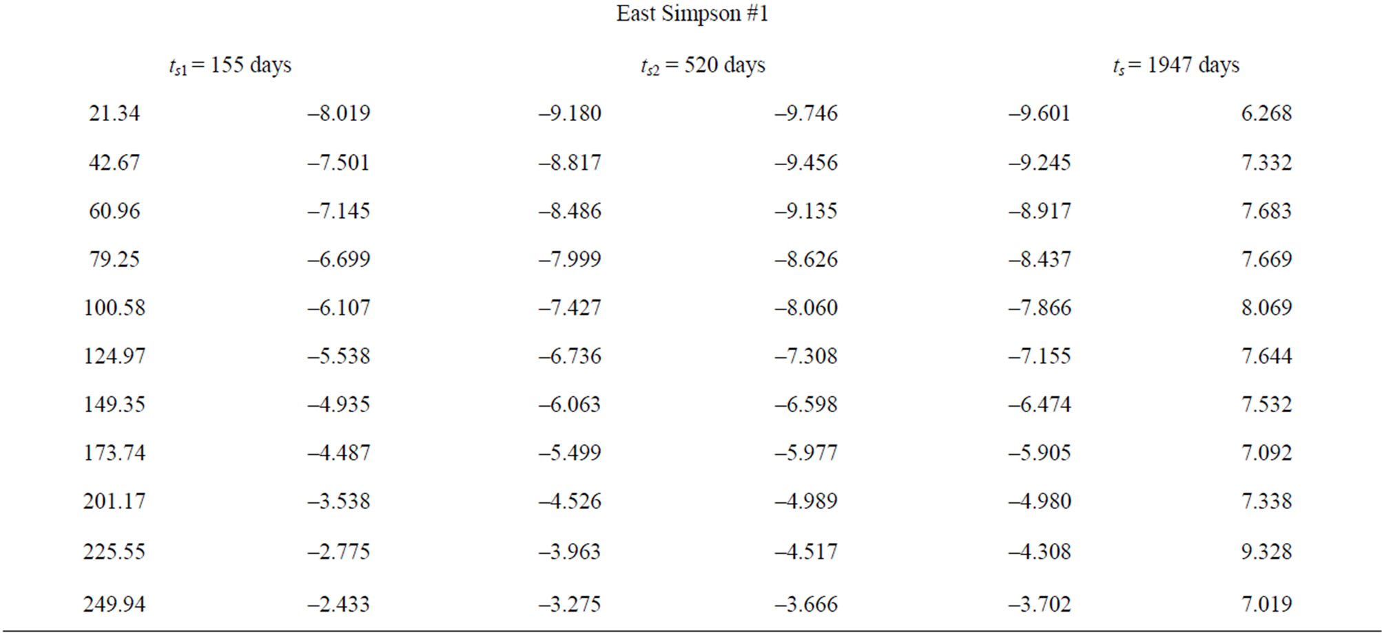
Table 2. Calculated values of A and B for wells Drew Point #1 and East Simpson #1.
that at values of ts = 2339 days and ts = 1947 days the values of Ts are close to the undisturbed temperature of formations, we can see from Table 2 that values of Ts and A are in good agreement. In Tables 3 and 4 we compare the calculated and measured shut-in temperature. The agreement between the values Teq and Ts is very good. US Geological Survey has obtained unique data for the well Put River N-1 (Table 5). Indeed, during two month of well’s shut-in five temperature logs were taken. For the well Put River N-1 we used values of ts1 = 34 days and ts2 = 66 days to estimate the empirical coefficients A and B.
In Table 6 we compare the calculated and measured shut-in temperatures for the well Put River N-1. In this case the difference between the calculated and measured temperatures is significant (Table 6). We can conclude that the shut-in times (34 and 66 days) are comparable with the formation freezeback period (Table 5). For this case we can use the suggested earlier a three-point method [9] for predicting the formation temperatures (Table 7). Here an additional temperature log (ts = 48 days) was used. From Table 7 follows that the agreement between calculated and measured temperatures is very good.
3. Temperature Gradient and Estimation of the Permafrost Thickness
In the permafrost areas the rate of heat flow at the frozen-unfrozen interface serves as the main criterion of the steadiness or non-steadiness of the thermal regime.
Let us assume that qt and qf are the heat flow density at the phase boundary in the unfrozen and frozen zone, respectively.
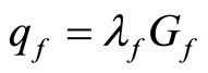
where λ is the thermal conductivity of geological formations.
It is clear that the condition qf = qu corresponds to a steady regime, the condition qf > qu corresponds to a regime of freezing and the condition qf < qu corresponds to a thawing regime. In addition, the change in the heat flow density at the permafrost base (frozen-unfrozen interface) is also an indicator of the climate change in the past [1]. When interpreted with the heat conduction theory, these sources can provide important information of patterns of contemporary climate change. For example, precision measurements in oil wells in the Alaskan Arctic indicate a widespread warming (2˚C - 4˚C) at the permafrost surface during the 20th century [6]. Thus to estimate values of qu and qf, it is necessary to determine the geothermal gradient and formation conductivity in the frozen and unfrozen sections of the wellbore. Unfortunately at present no methods are available for in-situ determination of formation conductivity. Samples of rocks are usually used to estimate formation thermal conductivity. Experimental studies show that λf > λu. For a given formation the λf > λu ratio is mainly a function of total water content [12]. The duration of the refreezing of the layer thawed during drilling is very dependent on the natural temperature of formation; therefore, the rocks at the bottom of the permafrost refreeze very slowly. In practice the position of the permafrost base (hp) is estimated by extrapolation. Let us examine the restoration of the natural temperature field by the example of the Bakhynay borehole 1-R [1]. The borehole was drilled for 23 months (1956 - 1958) to a depth of 2824 m. Nine temperature logs were performed over a shut-in period of 10 years, but the difference between the temperature of formations and that in the borehole was still greater than the measurement accuracy (0.03˚C - 0.05˚C). After a shut-in period of 1.5 years the thickness of permafrost was estimated as 470 m instead of 650 m. The restoration of the temperature regime was accompanied by formation of practically zero temperature gradient intervals (Figure 3). Therefore, if the shut-in time is insufficient, one may incorrectly attribute the zero temperature gradient intervals to some geological-geographical factors, an example of which in this case is the warming effect of the Lena River (the drilling site is the bank of the river). Below we present several examples of determination of the temperature gradients and evaluation of the permafrost thickness. For each section of the well we used a linear regression program to calculate the coefficients in the following equation
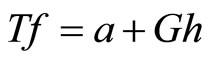
 (3)
(3)
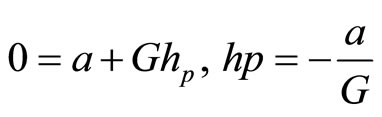
As can be seen for the section 21.34 - 249.94 m at ts = 520 days (Table 8) practically g = G (0.0267˚C/m). Similarly, for section 451.10 - 600.46 m at ts = 520 days the values g and G are very close (0.0408 and 0.0415˚C/m). Finally, the position of the permafrost base (hp) is estimated by extrapolation by using Equation (3) for Ts = 0˚C.
Therefore:
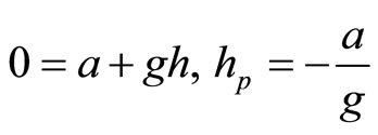 (4)
(4)
As can be seen the values of hp calculated for both sections of the well are in a good agreement (Table 8). In Table 9" target="_self"> Table 9 we present an example of data processing for two wells. As can be seen shut-in times of 155 days and 186 days do not enable to estimate the permafrost thickness with a sufficient accuracy. Earlier we developed “two temperature logs method” for determination the undisturbed formation temperatures.
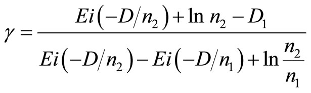
The working formulas are [13, p. 171]:
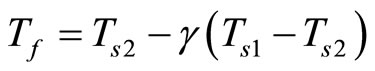 (5)
(5)
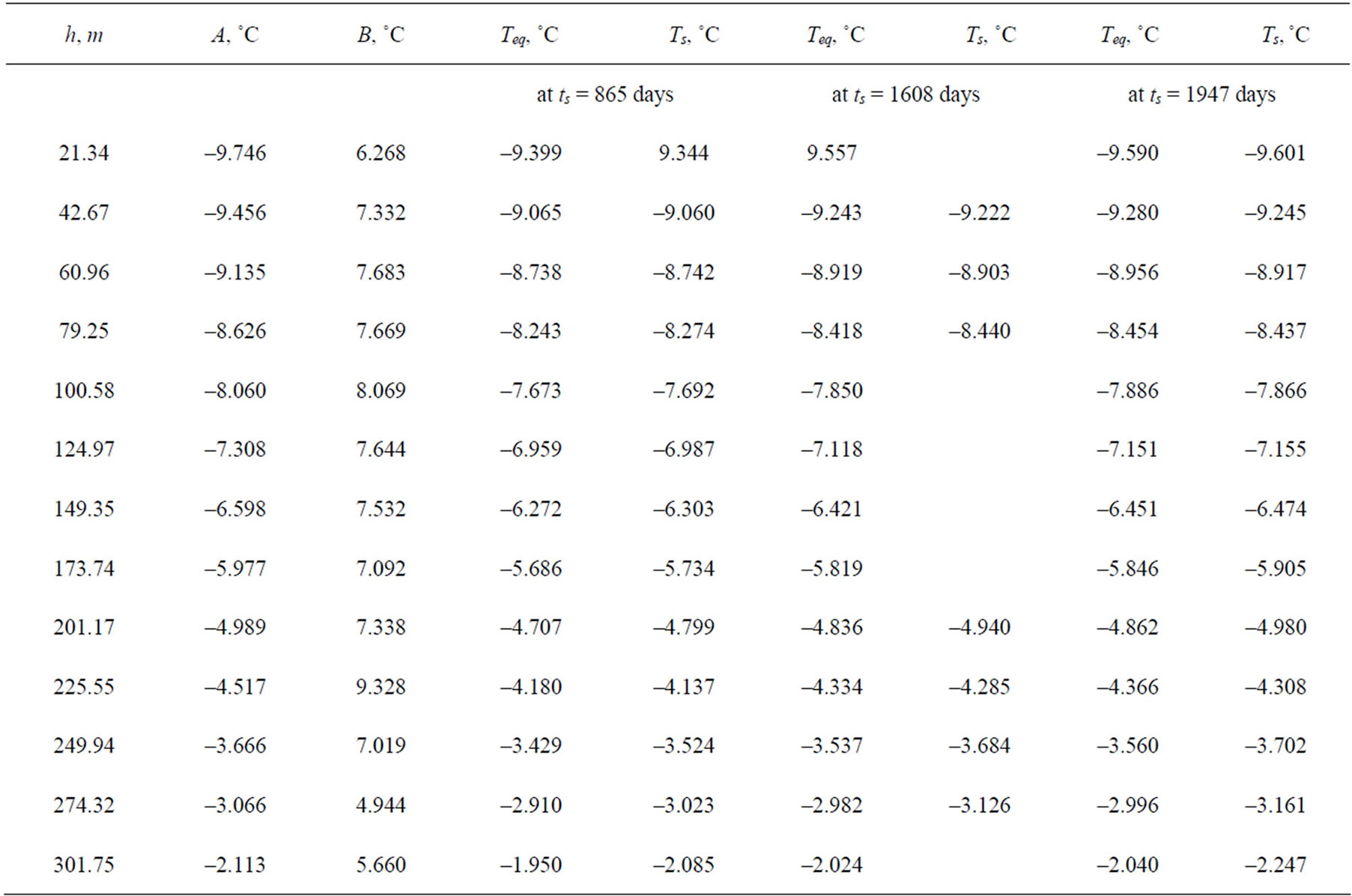
Table 3. Comparison of measured and observed shut-in temperatures, well East Simpson #1.
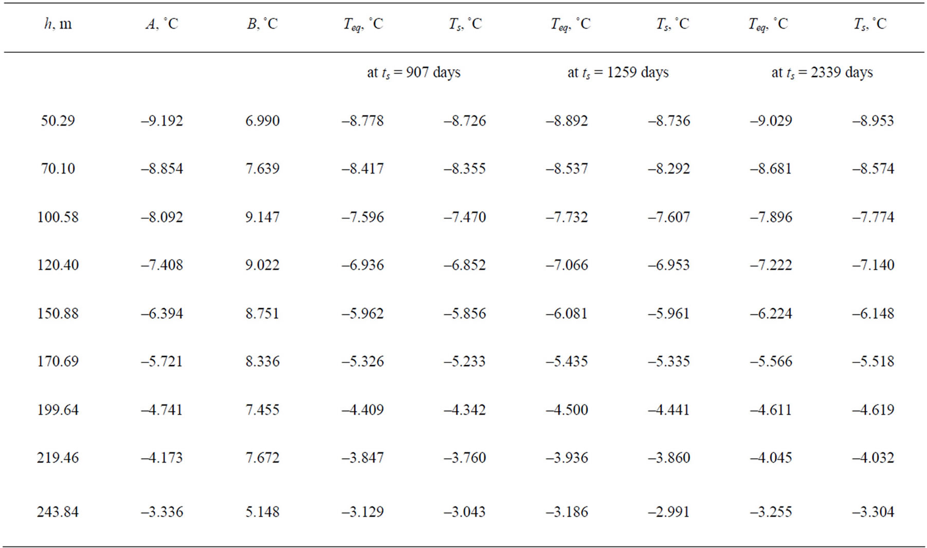
Table 4. Comparison of measured and observed shut-in temperatures, well Drew Point #1.
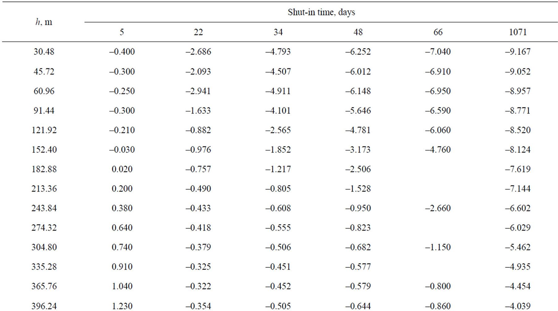

Table 5. Measured shut-in temperatures, well Put River N-1.
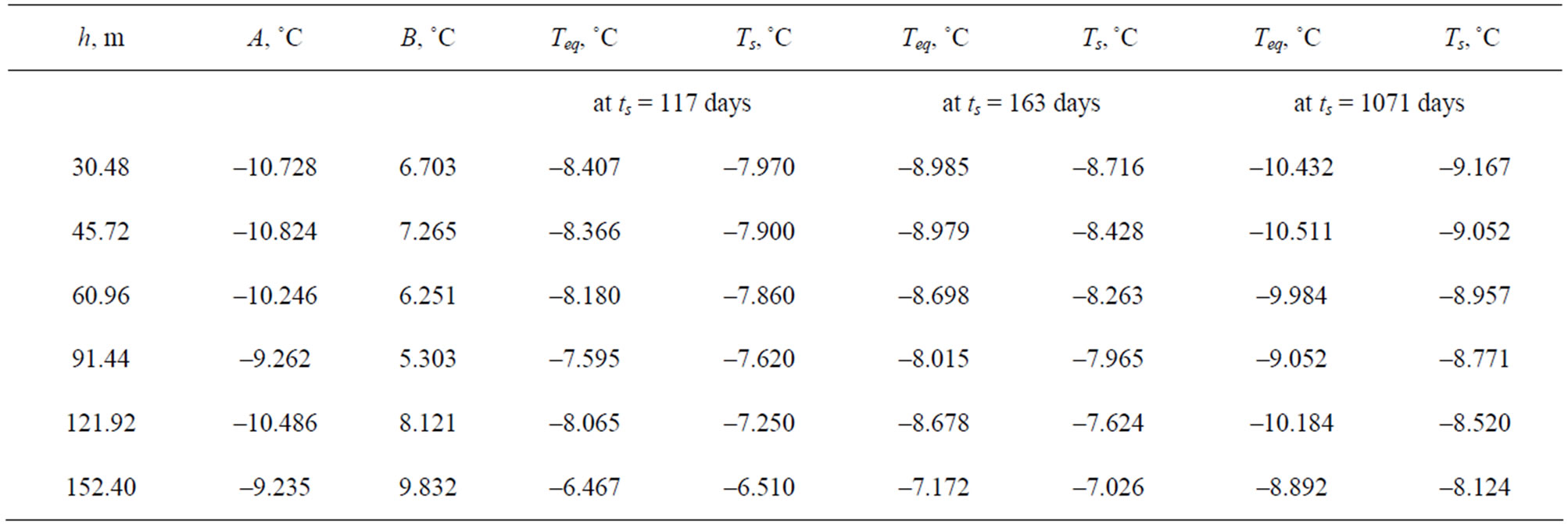
Table 6. Comparison of measured and observed shut-in temperatures, well Put River N-1.
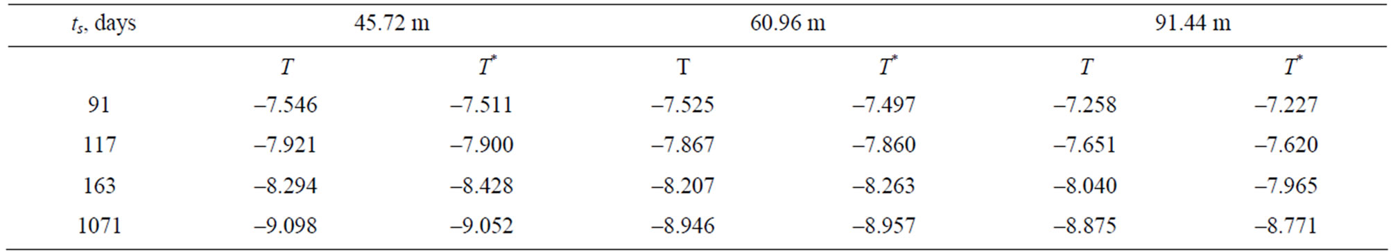
Table 7. Observed (T*) and calculated (T) shut-in temperatures (˚C) at three depths of the Put River N-1 well, Alaska; ts1 = 34, ts2 = 48, and ts3 = 66 days (after [9]).
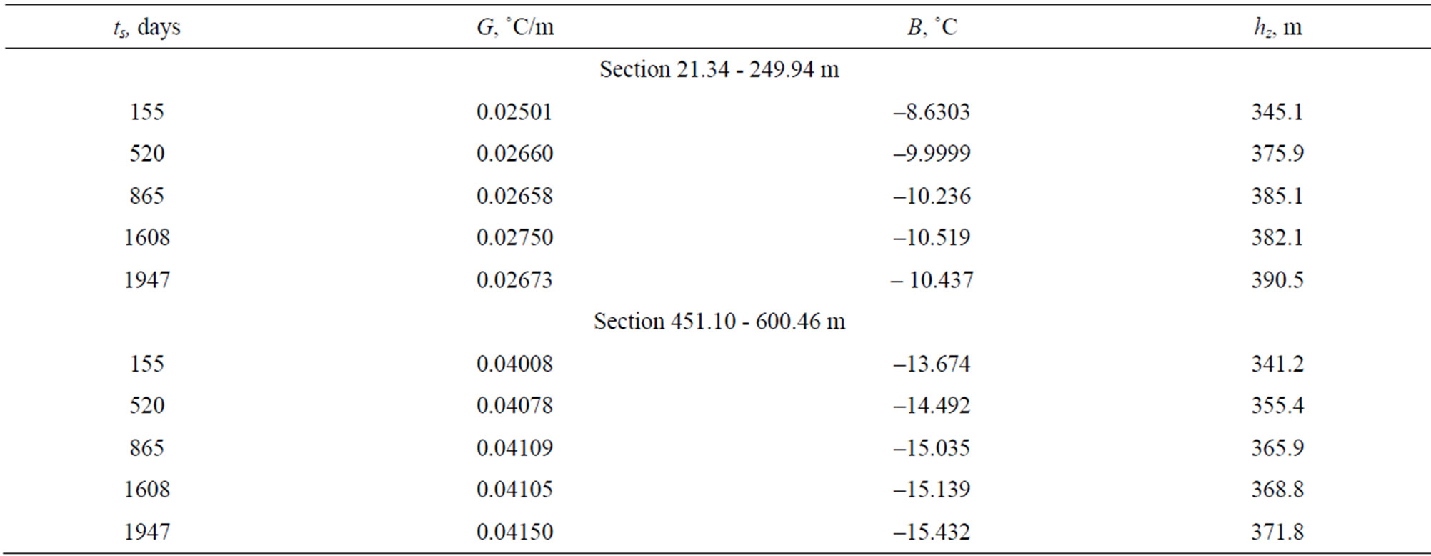
Table 8. The estimated values of permafrost thickness for two sections, East Simpson #1.

Table 9. An example of data processing for two wells.
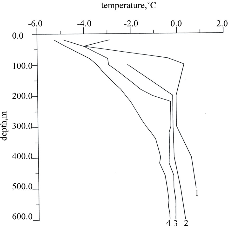
Figure 3. Restoration of temperature profile in the Bakhynay borehole 1-R (after [1]). Temperature surveys 1, 2, 3, and 4 were conducted at shut-in times of 0.4, 1.5, 3.4 and 10.4 years, respectively.
where

In Table 10 we present results of estimation of the formation temperature for two wells. And, finally, we use a linear regression program to determine the geothermal gradient (Table 11).
 (6)
(6)
The position of the permafrost base (hp) is estimated by extrapolation
Comparing the results of calculation hp (Table 9 at ts = 520 days and ts = 547 days) with that (Table 11) we can see the agreement between calculated values of hp is good.
4. Onset of Formations Freezeback
To plan the schedule of conducting temperature logs is important approximately to estimate the onset of the formations freezeback. Earlier we introduced term
“safety period”—the length of the shut-in period during which water-base mud remains free from freezing in permafrost areas [14]. From physical considerations it is clear that the “safety period” (tsp) can be determine from the condition Ts(tsp) = 0˚C (Figure 2). Thus, the time ts = tsp can be considered as the onset of the formations freezeback. The magnitude of the “safety period” depends mainly on the duration of the thermal disturbance (drilling time) and on the static temperature of permafrost. Precise temperature measurements (61 logs) conducted by the Geothermal Service of Canada in 32 deep shut-in wells in Northern Canada [2-5] were used to estimate the values of tsp [14]. The total drilling time (tt) for these wells ranged from 4 to 404 days, the total vertical depth (ht) ranged from 1356 m to 4704 m), and the depth of permafrost (hp) ranged from 74 m to 726 m. The range of formations temperatures was –0.5˚C > Tf > –4.6˚C.
We have found that the duration of the “safety period” tsp for a given depth can be approximated with sufficient accuracy as a function of two independent variables: time of thermal disturbance at the given depth (drilling time) and permafrost static temperature (Tf). A regression analysis computer program was used to process field data. It was revealed that the following empirical formula could be used to estimate the safety shut-in period:
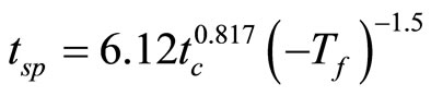 (7)
(7)
where tc is the thermal disturbance time (in days) at a given depth and temperature is inoc.
The value td is: , where th is the period of time needed to reach the given depth. The values of th can be determined from drilling records. The value td can be also estimated from Equation (2). Please note that in our paper [14] a safety factor of 2 was introduced in Equation (7). When planning to conduct a temperature log the condition ts >> tsp should be satisfied. We conducted calculations of tsp for the section 335.3 - 548.6 m, well Put River N-1 (Table 12). From Table 12 follows that for the temperature logs with ts = 5 days and ts = 22 days the condition ts >> tsp is not satisfied. As a result these temperature logs cannot be used for determination formation temperatures and estimation of the permafrost thickness. It should be remembered that in Equation (7), time is in days and temperature inoc.
5. Conclusion
It is shown that for large shut-in times the empirical Lachenbruch-Brewer formula can be used with good accuracy to estimate the shut-in temperatures. Only two temperature logs are needed to calculate the coefficients in the Lachenbruch-Brewer formula. Thus two temperature logs enable to predict formations temperatures, to determine the geothermal gradients, and to evaluate the thickness of
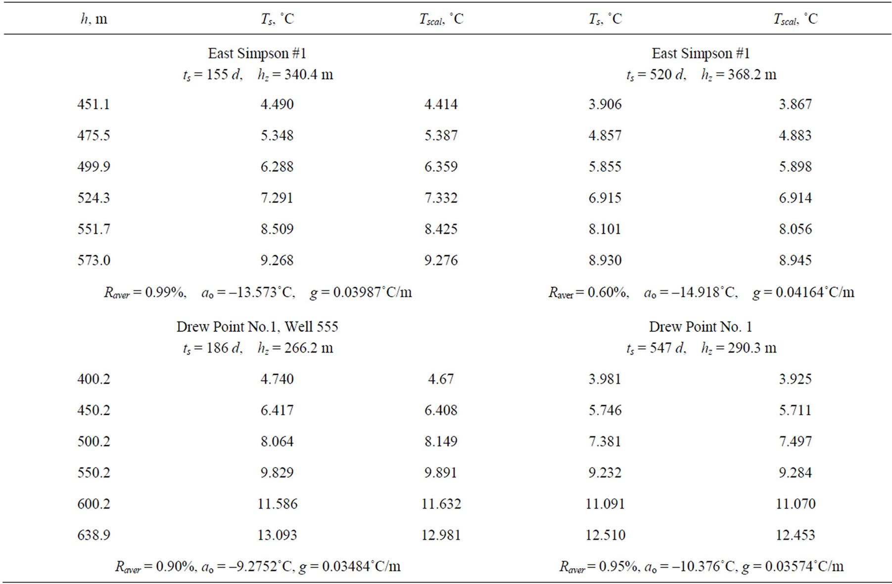
Table 9. An example of data processing for two wells.
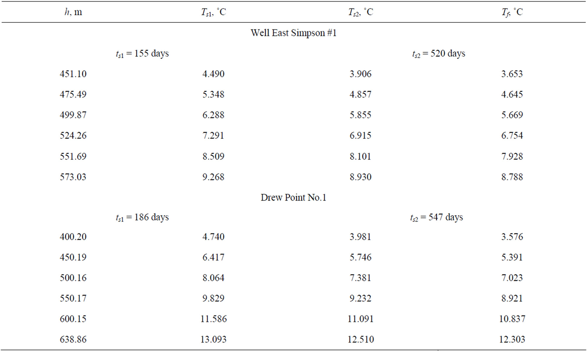
Table 10. Calculated formation temperatures by “two temperature logs method”.
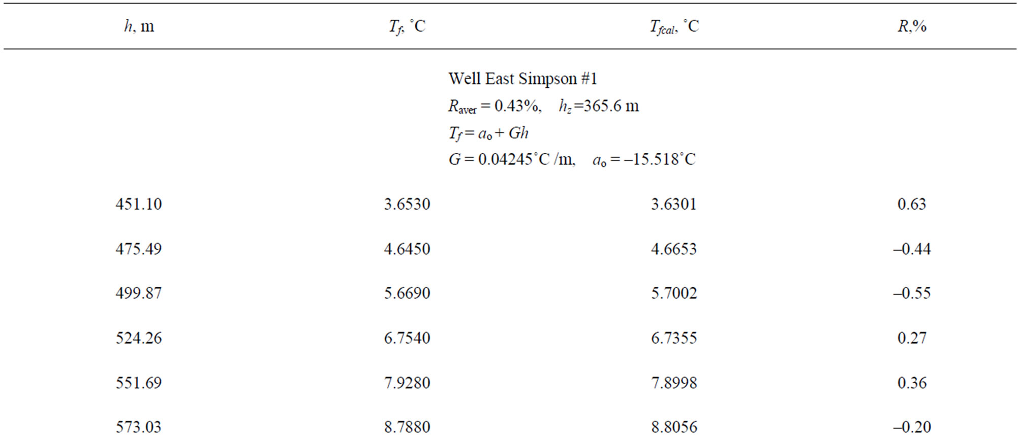
Table 11. Determination of the geothermal gradient, .
.
Table 12. The values of tsp for the section 335.3 - 548.6 m, well Put River N-1.
the permafrost zone. As a result the cost of monitoring the temperature regime of deep wells after shut-in can be drastically reduced. For short shut times (comparable with the time of complete freezeback) we suggest to utilize the “Three point method” [9]. The approximate evaluation of the onset of formations freezeback will assist in planning the schedule of conducting temperature logs.
6. Acknowledgements
The authors would like to thank an anonymous reviewer, who thoroughly reviewed the manuscript, and his critical comments and valuable suggestions were helpful in preparing this paper.
REFERENCES
- P. I. Melnikov, V. T. Balobayev, I. M. Kutasov and V. N. Devyatkin, “Geothermal Studies in Central Yakutia,” International Geology Review, Vol. 16, No. 5, 1974, pp. 565-568. HUdoi:10.1080/00206817409471838U
- A. E. Taylor and A. S. Judge, “Canadian Geothermal Data Collection-Northern Wells 1976-1977,” Geothermal Series, 10, Earth Physics Branch, Energy, Mines and Resources, Ottawa, 1977.
- A. S. Judge, A. E. Taylor and M. Burgess, “Canadian Geothermal Data Collection-Northern Wells 1977-1978,” Geothermal Series, 11, Earth Physics Branch, Energy, Mines and Resources, Ottawa, 1979.
- A. S. Judge, A. E. Taylor, M. Burgess and V. S. Allen, “Canadian Geothermal Data Collection—Northern Wells 1978-1980,” Geothermal Series, 12, Earth Physics Branch, Energy, Mines and Resources, Ottawa, 1981.
- A. E. Taylor, M. Burgess, A. S. Judge and V. S. Allen, “Canadian Geothermal Data Collection—Northern Wells 1981,” Geothermal Series, 13, Earth Physics Branch, Energy, Mines and Resources, Ottawa, 1982.
- A. H. Lachenbruch, T. T. Cladouhos and R. W. Saltus, “Permafrost Temperature and the Changing Climate,” Proceedings of the Fifth International Conference on Permafrost, Trondheim, 2-5 August 1988, pp. 9-17.
- I. M. Kutasov, “Prediction of Permafrost Thickness by the ‘Two Point’ Method,” Proceedings of the Fifth International Conference on Permafrost, Trondheim, 2-5 August 1988, pp. 965-970.
- N. A. Tsytovich, “The Mechanics of Frozen Ground,” Scripta Book Comp., Washington DC, 1975.
- I. M. Kutasov and L. V. Eppelbaum, “Prediction of Formation Temperatures in Permafrost Regions from Temperature Logs in Deep Wells-Field Cases,” Permafrost and Periglacial Processes, Vol. 14, No. 3, 2003, pp. 247-258. HUdoi:10.1002/ppp.457U
- A. H. Lachenbruch and M. C. Brewer, “Dissipation of the Temperature Effect of Drilling a Well in Arctic Alaska,” US Geological Survey Bulletin, Vol. 1083-C, 1959, pp. 74-109.
- “Boreholes Locations and Permafrost Depths,” Alaska, from US Geological Survey, 1998. http://nsidc.org/data/docs/fgdc/ggd223_boreholes_alaska
- V. T. Balobayev, “Geothermics of the Frozen Zone of the Lithosphere of the Northern Asia,” Nauka, Novosibirsk, 1991.
- I. M. Kutasov, “Applied Geothermics for Petroleum Engineers,” In: Development in Petroleum Science, Elsevier, 1999.
- I. M. Kutasov and D. G. Strickland, “Allowable Shut-In Is Estimated for Wells in Permafrost,” Oil and Gas Journal, 1988, pp. 55-60, OSTI ID: 6765096.
Nomenclature
A, B—Empirical coefficients (Equation (1));
a—Parameter (Equations (3) and (6));
G—Geothermal gradient;
g—Temperature gradient;
ht—Total well depth;
h—Depth;
hp—Depth to base of ice-bounded permafrost;
Teq—Shut-in temperature predicted by Lachenbruch- Brewer formula;
Tf—Formation temperature;
Ts—Shut-in temperature;
t—Time;
tc—Time of “thermal disturbance” at a given depth;
tt—Otal drilling time;
ts—Shut-in time;
tep—Time of the thawed formation refreezing;
tsp—Onset of the formation freezeback.
Greek Symbols
λ—Thermal conductivity of formations.
Subscripts
u—Unfrozen;
f—Frozen.