World Journal of Nuclear Science and Technology
Vol.07 No.02(2017), Article ID:75821,18 pages
10.4236/wjnst.2017.72009
Numerical Analysis for Transients in External Source Driven Reactors
Willian Vieira de Abreu1, Alessandro da Cruz Gonçalves2, Zelmo Rodrigues de Lima1*
1Nuclear Engineering Institute, National Commission for Nuclear Energy, Rio de Janeiro, Brazil
2Nuclear Engineering Program, COPPE, Federal University of Rio de Janeiro/UFRJ, Rio de Janeiro, Brazil

Copyright © 2017 by authors and Scientific Research Publishing Inc.
This work is licensed under the Creative Commons Attribution International License (CC BY 4.0).
http://creativecommons.org/licenses/by/4.0/


Received: February 23, 2017; Accepted: April 25, 2017; Published: April 30, 2017
ABSTRACT
The main purpose of this paper is to perform a numerical analysis of the Neutron Spatial Kinetic Equations, subject to transients of the External Neutron Source, by applying the Implicit Euler Method as well as the Runge-Kutta Method in order to check which methods are best applicable in transients caused by External Neutron Source. For this purpose, a one-dimensional ADS reactor with a constant external source was simulated based on the geometry of ANL-BSS-6 reactor for benchmark effects.
Keywords:
ADS, Transients, Spatial Kinetics

1. Introduction
One of the society main concerns refers to the management of nuclear waste, which are generated at every stage of the fuel cycle. High-Activity Waste (HLW) are composed of fission products and transuranic elements, generated in the reactor core, and they can last a half-life of thousand years. However, the advent of the hybrid reactor concept, also known as “Accelerator-Driven System” (ADS), has opened the possibility that such waste can be reused in the future, after being reprocessed [1] [2] .
The hybrid systems [3] , designed by the researcher Carlo Rubbia, Physics Nobel Prize in 1984, couples a particle accelerator and a subcritical nucleus. Quite a few proposals take for granted a proton accelerator, transmitting a continuous beam with energy around 1 GeV. The accelerator can be linear (linac) or circular (cyclotron). High-power accelerators are in constant development, and building machines with specific needs, as for example, with electric efficiency close to 50% and bundles with power up to 10 MW for cyclotrons and up to 100 MW for linacs now seems feasible.
The protons are injected onto a spallation target, producing a source of neutrons to propel the subcritical nucleus. The target is made of solid heavy metal or of liquid-metal. The reactions of the spallation on the target issue from ten to twenty neutrons per incident proton, which are introduced into the subcritical nucleus inducing future nuclear reactions. Except for the subcritical state, the core of the reactor is very similar to that of a critical one [4] . Moreover, the ADS can be designed to operate on both thermal or fast neutron spectra.
Hybrid reactors, such as ADSs, have attracted world attention and are objects of research and development in many countries [5] . Japan, the USA and France are currently building pilot plants to demonstrate the efficiency of hybrid reactors in the process of lifetime reduction of HLW. These types of reactors are not only used for the transmutation of transuranic elements, but they can be used for power generation.
Hybrid reactors consist of intrinsically safe systems, so that the chain reaction inside them is not self-sustainable, and it can be interrupted simply by shutting off the proton accelerator simply, which demonstrates a straightforward relationship between the external source and the reactor control.
Therefore, this article brings forward a numerical analysis of the spatial kinetic equations subject to transients caused by the external source of neutrons, that of a one-dimensional ADS reactor.
2. Accelerator-Driven System Kinetics
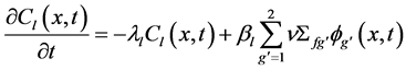
A model of one-dimensional multi-group diffusion dependent on the time considering delayed neutrons is used to study the kinetic of the ADS reactor subject to transients caused by external source of neutrons. The spatial kinetic neutron diffusion equations, for two energy groups, six delayed neutron precursor groups and with the presence of an external source are written as follows:
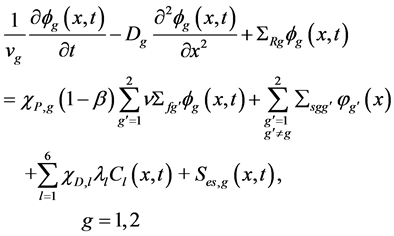 (1)
(1)
 (2)
(2)
where  is the neutron flux,
  the diffusion coefficient,
  the removal cross section,
  the average number of neutrons emitted by fission multiplied by fission cross section,
  the scattering cross section,
 the external source, defined in the group g of energy,
  the delayed neutron precursor concentration in precursor group l, all defined at point
  and time t,
  the velocity,
  the fission spectrum for prompt neutrons, both in group g,
  the fission spectrum for delayed neutrons,
  the decay constant,
  the fraction of all fission neutrons emitted per fission, defined in the l precursor group and finally
  the total fraction of fission neutrons which are delayed. Equations (1) and (2) are discretized in space and time, as described below.
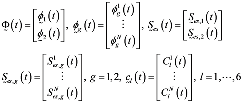
2.1. Spatial Discretization
The spatial discretization scheme adopted is based on classical formulation of finite differences, implemented in the box schema [6] [7] . Therefore, Equations (1) and (2) can be rewritten in the following matrix form:
 (3)
(3)
 (4)
(4)
where
 (5)
(5)
where  is a block-tree-diagonal matrix representing the leakage and removal,
  and
and  are, respectively, the fission and scattering block diagonal matrices, and
 (6)
(6)
with  being the total number of boxes. The system Equations (3) and (4) stands for the semi-discretized form.
2.2. Time Dependent Solution
In order to solve time dependent equation system, the analytical integration procedure [8] has been adopted for the precursor concentration equation, Equation (4), whereas the Methods Implicit Euler and Rosenbrock Generalized Runge-Kutta with automated time step size control [9] [10] [11] are considered for the neutron flux in Equation (3).
2.2.1. Analytical Solution of the Delayed Neutron Precursor Equation
In the analytical integration, it was assumed that the term fission rate varies linearly between times  to
to  in Equation (4), which was analytically integrated in this interval, thus obtaining the expression for
  in
in :
:
 (7)
(7)
where coefficients  and
and  are defined as:
 (8)
(8)
2.2.2. Implicit Euler
The implicit Euler method applied to the matrix equation, Equation (3), leads to the following expression:
 (9)
(9)
Replacing Equation (7) in Equation (9) the result is the following system of linear equations:
 (10)
(10)
where the blocks of matrix are given for:
 , (11)
 , (12)
 , (13)
 , (14)
 , (15)
 , (16)
 , (17)
2.2.3. Rosenbrock Generalized Runge-Kutta Method
The solution to Equation (7) is given, by Rosenbrock method by:
 . (18)
where the correction vectors  are obtained by solving the following system of equations:
 .(19)
.(19)
where  and
and  are, respectively, the Jacobian and the right side of the linear system, and coefficients
 , ds,
, ds,  and
and  are constants fixed, independent of the problem, where the chosen values are those adopted by Kaps-Rentrop [9] and by Shampine [12] . The four solutions of the above equations,
  , are calculated through a L-U matrix decomposition
 , followed by four backward substitutions.
During the implementation of the automatic time step size control two solutions of Equation (18) are used: a third order solution,  , with different coefficients
 ,
,  , but with the same
 , and a real fourth order solution
 . The estimate of the local truncation error is given by:
 (20)
(20)
and the equation applied to automatically adjust time step size is:
 (21)
(21)
where  is the projected step size for the next step,
  is the step in the previous time, 0.9 a safety factor,
  the estimated local truncation error and
  a tolerance provided by the user. Besides,
  is limited by the interval
 , to reduce the number of rejected steps and avoid a zigzag behavior. The process can be synthesized in the following way: if a time step in the integration is successful, that is, if
 , then the fourth order solution of Equation (18) is accepted and the next time step is chosen according to Equation (21) and proceeds in time. However, if the time step size test fails, that is, if
 , the solution is rejected, and then the previous time steps is repeated using a time step size reduced through Equation (21), until the condition
  is satisfied.
3. Results and Discussion
In order to test the related numerical methods, computational codes programmed in the FORTRAN language were implemented. For the implicit method of Euler, a computational code called KDF1D2GIE was developed, whereas for the Runge-Kutta method a computational code was developed called KDF1D2GRK. Both codes solve the spatial kinetics equations with or without external neutron source for a one-dimensional, multi-region, and two energy groups. In addition, a computational code called DF1D2G was developed to solve the stationary diffusion equation, providing the neutron fluxes and the multiplication factor. For purposes of comparison the implicit Euler method was considered the reference method. Before simulating the transients associated with the external source of an ADS reactor, codes DF1D2G, KDF1D2GIE and KDF1D2GRK were validated considering a known benchmark, as follows in the next section.
3.1. Validation of Numerical Methods
To test the presented methods, the ANL-BSS-6 benchmark [13] [14] was considered a problem of one-dimensional slab infinite for transients in spatial kinetics, with three regions, and the regions I and III are 40 cm long, both with the same nuclear parameters and a central region, 160 cm long, as shown in Figure 1. Nuclear and kinetic parameters are listed in the Table 1 and Table 2.
At first a stationary calculation was performed by using the DF1D2G code to solve the neutron diffusion equation for two energy groups, thus obtaining the fast and thermal neutron fluxes, which will be used as the initial condition of the transient problems, and a multiplication factor  equal to 0.9016 (according [14] the reference value for the
  is equal to 0.90155). The fluxes of neutrons were normalized considering a power per unit area equal to 87 KW/cm2.
The ANL-BSS-6 benchmark presents two cases different from transients: A1 and A2. In both cases, the KDF1D2GIE and KDF1D2GRK codes were performed considering the same spatial discretization with a 1 cm mesh. In the simulation of the transient with the KDF1D2GIE code a time step size of 0.001 s was adopted, while the KDF1D2GRK code considered the two options of numerical parameters: Kaps-Rentrop (KR) and Shampine (S) and was used in Equation

Figure 1. ANL-BSS-6 benchmark geometry.

Table 1. Nuclear parameters.
Table 2. Kinetics parameters.
Speeds:  and
and .
.
(21) a tolerance equal to 0.001. Moreover, the neutron fluxes obtained by the implicit Euler method and the Runge-Kutta method were also compared at time 1, 2, 3 and 4 s, considering the definition of relative percentage error is given by:
 . (22)
3.1.1. ANL-BSS-6-A1 Case
In this case the thermal absorption cross section in the first region is increased linearly in 3% up to 1 s, and maintained constant up to 4 s. Figure 2 and Figure 3 illustrate the behavior of the fast and thermal neutron fluxes at the 1 s and 4 s instants of the transient. Figure 4 shows the evolution in time of power per unit area during the simulation of 4 s. It can be seen from these graphs that the methods practically reproduce the same results and that they are in agreement with
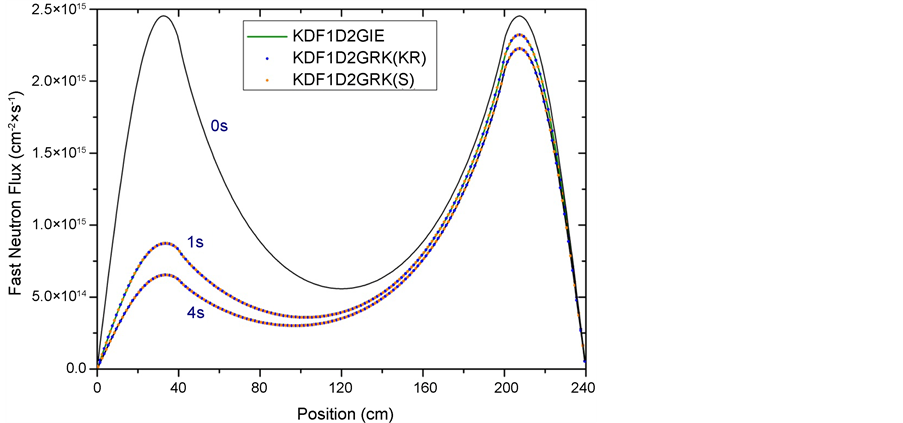
Figure 2. ANL-BSS-6-A1 case―fast neutron flux.
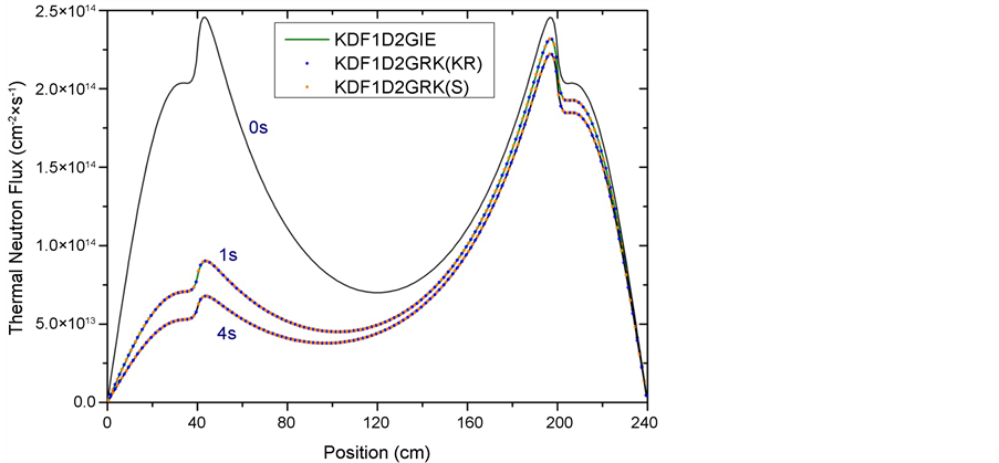
Figure 3. ANL-BSS-6-A1 case―thermal neutron flux.
the reference solution presented in [14] . Considering the instants in 1, 2, 3 and 4 s, the highest value for the percentage relative error using the Kaps-Rentrop parameters, when compared to the implicit Euler method, was 0.163%, obtained at the instant of 4 s in the thermal flux. Using the Shampine parameters, the largest percentage relative error was 0.182%, occurring in 1s, also in the thermal flux. Regarding the processing time, Table 3 shows that the KDF1D2GIE code presented a 54.6% less time in relation to the time of the KDF1D2GRK code, with the Kaps-Rentrop parameters, and 31.7% less than the processing time with the parameters of Shampine. While this last option processed in a 33.6% lower time compared to the option with the Kaps-Rentrop parameters.
3.1.2. ANL-BSS-6-A2 Case
In the second case the thermal absorption cross section in the first region is reduced linearly in 1% up to 1 s, and maintained constant up to 4 s. Figures 5-7 show, respectively, the behavior of the neutron fluxes in the instants in 1 s and 4 s and the evolution in the time of the power per unit area during the simulation of 4 s. As in case A1, it can be seen from these graphs that the methods obtained very close results and that they are also in agreement with the reference solution presented in [14] . Considering the instants in 1, 2, 3 and 4 s, the highest value of the percentage relative error using the Kaps-Rentrop parameters was 0.524%, at the instant in 1 s and in the thermal flux, whereas for the Shampine parameters it was 0.8% also in 1 s and in the thermal flux.
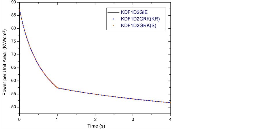
Figure 4. ANL-BSS-6-A1 case―evolution in time of power per unit area.
Table 3. Processing time (s).
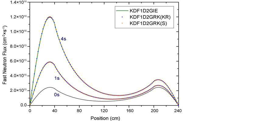
Figure 5. ANL-BSS-6-A2 case―fast neutron flux.
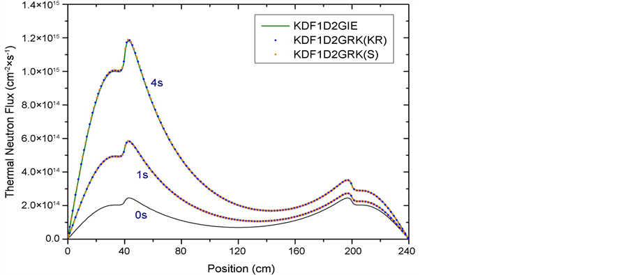
Figure 6. ANL-BSS-6-A2 case―thermal neutron flux.
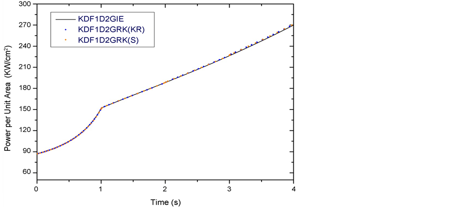
Figure 7. ANL-BSS-6-A2 case―evolution in time of power per unit area.
With respect to the processing time, according to Table 3, and unlike case A1, the KDF1D2GIE code required more time: 31% slower than KDF1D2GRK with Kaps-Rentrop parameters and 42.6% slower In relation to the Shampine parameters, being this parameter option 16.6% faster than the Kaps-Rentrop option.
3.2. Analysis of Transients in an ADS
In this section, the Implicit Euler method and the generalized Runge-Kutta method were used to analyze some types of transients caused by the external neutron source in a one-dimensional ADS reactor, in order to verify which methods are more efficient in convergence and computation time.
The one-dimensional ADS reactor has its geometry and nuclear and kinetic parameters based on the ANL-BSS-6 benchmark reactor, in which case an external source of neutrons located geometrically in the center of the reactor and with a length of 4 cm, as shown in the Figure 8. This source of neutrons, which represents the source of spallation that is bombarded by a proton beam, can be approximated as a source of constant intensity because the proton beam employed in ADS reactors operates at a very high frequency, above 170 MHz. In the cases of transients that will be approached in the next sections, an external neutron source with a constant intensity equal to 1014 neutrons/s was used.
Using the KDF1D2GIE and KDF1D2GRK codes, three types of transients associated with an ADS reactor will be simulated and will focus on the proton accelerator perturbations, causing variations in the intensity of the proton beam and consequently the intensity of the external source of neutrons. The first transient concerns the activation of the proton accelerator when the ADS reactor is in zero power level condition. The second transient corresponds to the interruption in the proton beam for a short period of time and the third transient to be addressed describes the occurrence of a power peak in the proton beam. These last two transients were based on the cases studied in [15] . In order to simulate the transients, the same spatial discretization of the previous section was considered, with a mesh of 1 cm and for the KDF1D2GIE code the same time step size was adopted: 0.001 s. For the KDF1D2GRK code, a tolerance equal to 0.1 was used in Equation (21).
3.2.1. Source of Neutrons Start
The switching on of the proton accelerator to start the ADS reactor can be considered an operational transient. The external source of neutrons begins to emit
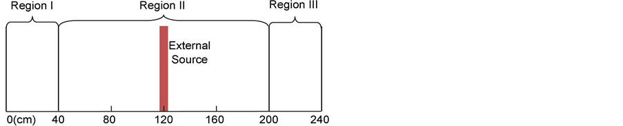
Figure 8. Reactor ADS geometry unidimensional.
neutrons at the initial instant, t = 0 s, and after some time the generated neutron flux reaches an asymptotic behavior. The simulation was performed for 20 s and Figures 9-11 show, respectively, the behavior of the neutron fluxes at these instant and the evolution in the time of the power per unit area during the simulation.
In the time in 20 s, the highest percentage relative error, when comparing the results of KDF1D2GIE with KDF1D2GRK using the Kaps-Rentrop parameters was 0.163%, in the fast and thermal fluxes, whereas for the Shampine parameters it was 0.189% also in the fast and thermal fluxes. Regarding the processing time, Table 4 shows that the KDF1D2GIE code presented a 41.2% longer time in relation to the KDF1D2GRK code time, with the Kaps-Rentrop parameters, and 8.8% higher than the processing time with the parameters of Shampine. The option with the Kaps-Rentrop parameters processed in a 35.6% less time compared to the option with the Shampine parameters.
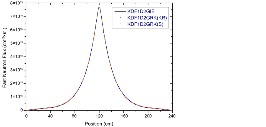
Figure 9. Reactor ADS―source of neutrons start―fast neutron flux.
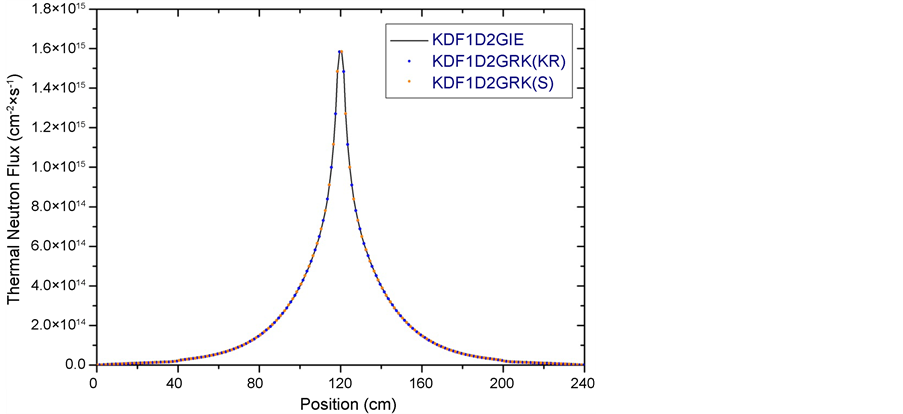
Figure 10. Reactor ADS―source of neutrons start―thermal neutron flux.
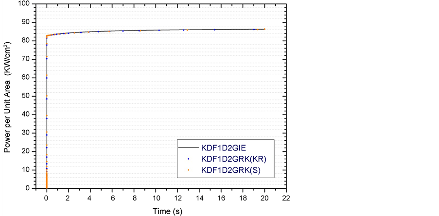
Figure 11. Reactor ADS―evolution in time of power per unit area.
Table 4. Processing time (s).
In this transient the external source of neutrons is switching on instantaneously and this impacts, practically, in the same way in the power per unit area. As can be seen in Figure 10, the power per unit area varies sharply in milliseconds. It has been signed up, for example, that by code KDF1D2GIE, in 1 ms, after switching on the external source of neutrons, the power per unit area reached a value close to 65 KW/cm2, which corresponds to 75% of the nominal value, equal to 87 KW/cm2. Whereas, with the code KDF1D2GRK, at the same time, it reached 93% of the nominal value.
3.2.2. Accelerator Beam Interruption
In this transient the reactor is operating critically and the proton beam of the accelerator is interrupted in the instant in 1 s and after 2 s over the beam is reconnected. Figure 12 and Figure 13 illustrate the behavior of the fast and thermal neutron fluxes at the instant in 1 s, at the beginning of the ABI, and Figure 14 and Figure 15 show the fast and thermal neutron fluxes at the instant in 3 s, at the end of the ABI. Considering the instants in 1 s and 3 s, the highest percentage relative error, when comparing the KDF1D2GIE and KDF1D2GRK codes, using the Kaps-Rentrop parameters was 0.072% in the thermal flux, occurring in 3 s, while for The Shampine parameters were 0.093% in the fast flux, occurring in 1 s. Table 4 shows that the code KDF1D2GRK with the parameters of Shampine was the fastest: 45.9% in relation to the option with Kaps-Rentrop parameters and 24.7% in relation to KDF1D2GIE.
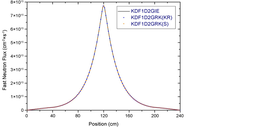
Figure 12. Reactor ADS―ABI―fast neutron flux, t = 1 s.

Figure 13. Reactor ADS―ABI―thermal neutron flux, t = 1 s.
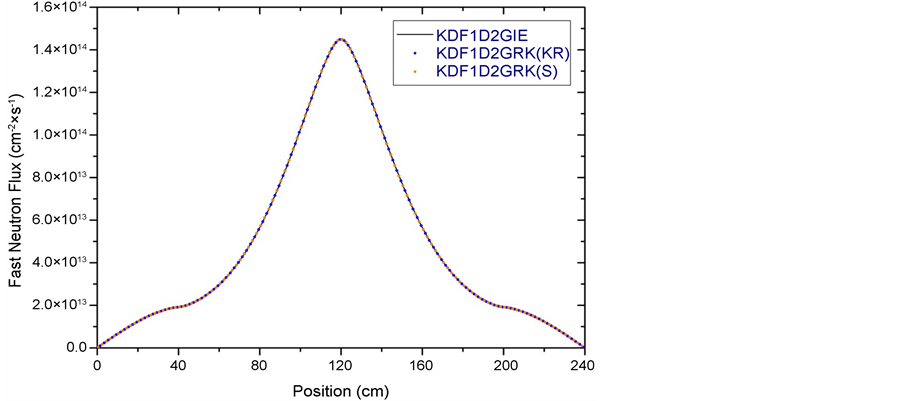
Figure 14. Reactor ADS―ABI―fast neutron flux, t = 3 s.
Figure 16 shows the behavior of the power per unit area, considering a simulation with the duration of 10 s. With the interruption of the proton beam at the instant in 1 s an abrupt change in power is observed and the same occurs with the throttle drive in 3 s. It is also observed that between these instants, the power is reduced slowly due to the sub-criticality of the ADS reactor. Figures 12-15 also show the reduction in the intensity of the neutron fluxes between these instants.
3.2.3. Accelerator Beam Over-Power
In this transient the reactor is operating critically and the intensity of the proton beam of the accelerator is increased by 100% instantaneously and after 2 s over the beam has its intensity restored to the initial level. Figure 17 and Figure 18
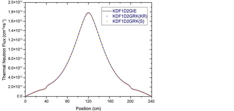
Figure 15. Reactor ADS―ABI―thermal neutron flux, t = 3 s.
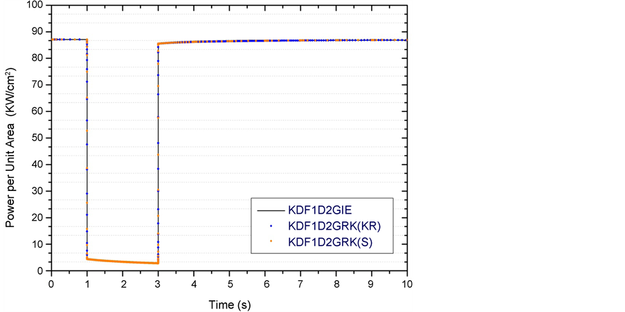
Figure 16. Reactor ADS―ABI―evolution in time of power per unit area.

Figure 17. Reactor ADS―ABO―fast neutron flux, t = 1 s.
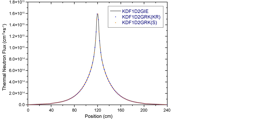
Figure 18. Reactor ADS―ABO―thermal neutron flux, t = 1 s.
show the behavior of the fast and thermal neutron fluxes at the instant in 1 s, at the beginning of ABO, and Figure 19 and Figure 20 show the fast and thermal neutron fluxes at the instant in 3 s, at the end of ABO. Considering these instants in 1 s and 3 s, the highest percentage relative error, when comparing the KDF1D2GIE and KDF1D2GRK codes, using the Kaps-Rentrop parameters was 0.093%, in the fast flux, occurring in 1 s, while for the Shampine parameters were 0.044% in the fast and thermal fluxes, occurring in 3 s. It can be observed, as in the previous case and Table 4, that the code KDF1D2GRK with the parameters of Shampine was the fastest: 35.2% in relation to the option with the parameters of Kaps-Rentrop and 20.7% in relation to KDF1D2GIE.
The behavior of the power per unit area in the transient ABO, considering a simulation with the duration of 10 s can be verified in Figure 21. With the increase in the intensity of the proton beam of the accelerator in the instant in 1 s

Figure 19. Reactor ADS―ABO―fast neutron flux, t = 3 s.

Figure 20. Reactor ADS―ABO―thermal neutron flux, t = 3 s.
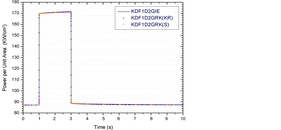
Figure 21. Reactor ADS―ABO―evolution in time of power per unit area.
observes a variation of power, going from 87 KW/cm2 to around 170 KW/cm2. With the accelerator operating at normal intensity, the ADS reactor operates at criticality and therefore, with an increase in beam intensity, the reactor starts operating on super criticality. Thus, a gradual increase in power between the instants of 1 s and 3 s can be observed. Figures 17-20 also show the corresponding increase in neutron flux intensity between these instants.
4. Conclusions
In this work the solution of the spatial kinetics equations for ADS reactors was presented. The spatial kinetics equations were discretized in the spatial variable considering the finite difference method. In order to solve the time-dependent part, the implicit Euler method and the Runge-Kutta method were used, which were implemented in computational codes based on the Fortran language. The implicit method of Euler did not consider an automatic adjustment in the time step. While the code developed for Runge-Kutta was developed considering a truncation error monitoring scheme to automatically adjust the size in the time step. The codes were tested and validated in a well-known benchmark for one- dimensional transients. Both codes were satisfactory in the transient simulations for the ADS reactor involving fluctuations in the external neutron source, and the Runge-Kutta method using the numerical parameters of Shampine proved to be the most efficient in the processing time.
It is intended to implement the Runge-Kutta method in more complex geometries for the ADS reactors, using a three-dimensional geometry and considering a more detailed description of the spallation source. It is also relevant in the future to consider the effects of thermohydraulic feedback because it has been found that the transients of the external neutron source cause strong variations in the power of the reactor in milliseconds and this is likely to impact on the reactivity coefficients.
Acknowledgements
The authors are grateful for the support provided by the Fundação Carlos Chagas Filho de Amparo à Pesquisa do Estado do Rio de Janeiro (FAPERJ), Brazil.
Cite this paper
de Abreu, W.V., Gonçalves, A.C. and de Lima, Z.R. (2017) Numerical Analysis for Transients in External Source Driven Reactors. World Jour- nal of Nuclear Science and Technology, 7, 103-120. http://doi.org/10.4236/wjnst.2017.72009
References
- 1. Salvatores, M., et al. (1997) Long-Lived Radioactive Waste Transmutation and the Role of Accelerator Driven (Hybrid) Systems. Nuclear Instruments and Methods, 414, 5.
- 2. Lomonaco, G., Frasciello, O., Osipenko, M., Ricco, G. and Ripani, M. (2014) An Intrinsically Safe Facility for Forefront Research and Training on Nuclear Technologies—Burnup and Transmutation. The European Physical Journal Plus, 129, 74.
https://doi.org/10.1140/epjp/i2014-14074-6 - 3. Rubbia, C., et al. (1995) Conceptual Design of a Fast Neutron Operated High Power Energy Amplifier. CERN Report, Genebra.
- 4. Yasin, Z. and Shahzad, M.I. (2010) From Conventional Nuclear Power Reactors to Accelerator-Driven Systems. Annals of Nuclear Energy, 37, 87-92.
- 5. Organization for Economic Co-Operation and Development and Nuclear Energy Agency (2002) Accelerator-Driven Systems (ADS) and Fast Reactors (FR) in Advanced Nuclear Fuel Cycles: A Comparative Study. Technical Report, Paris.
- 6. Nakamura, S. (1977) Computational Methods in Engineering and Science. Wiley and Sons, New York.
- 7. Alvim, A.C.M. (2007) Métodos Numéricos Em Engenharia Nuclear. Certa Ltd., Curitiba.
- 8. Stacey, W.M. (1969) Space-Time Nuclear Reactor Kinetics. Academic Press, New York.
- 9. Kaps, P. and Rentrop, P. (1979) Generalized Runge-Kutta Methods of Order Four with Stepsize Control for Stiff Ordinary Differential Equations. Numerische Mathematik, 33, 55-68.
https://doi.org/10.1007/BF01396495 - 10. Press, H.W., Teukolsky, S.A., Vetterling, W.T., et al. (1992) Numerical Recipes in Fortran. 2nd Edition, Cambridge University Press, London.
- 11. Aviles, B.N. (1993) Development of a Variable Time-Step Transient NEM Code: SPANDEX. Transactions of the American Nuclear Society Journal, 68, 425-427.
- 12. Shampine, L.F. (1982) Implementation of Rosenbrock Methods. ACM Transactions on Mathematical Software, 8, 94.
https://doi.org/10.1145/355993.355994 - 13. Nagaya, Y. and Kobayashi, K. (1995) Solution do 1D Multi-Group Time-Dependent Diffusion Equations Using the Coupled Reactors Theory. Annals Nuclear Energy, 22, 421-440.
- 14. Argonne Code Center (1977) Benchmark Problem Book. Argonne National Laboratory, Chicago.
- 15. Figueira, A.J., Alvim, A.C.M. and da Silva, F.C. (2016) Non Symmetric Alternating Direction Explicit Method Applied to the Calculation of ADS Transients, Annals of Nuclear Energy, 90, 459-467.