World Journal of Nuclear Science and Technology
Vol.3 No.1(2013), Article ID:27522,6 pages DOI:10.4236/wjnst.2013.31004
Data Evaluation and Visibility in Single Beam Scanner of Gamma Ray Tomography
1Department of Nuclear Energy, Federal University of Pernambuco, Recife, Brazil
2Department of Mechanical Engineering, Federal University of Pernambuco, Recife, Brazil
3Informatics Center, Federal University of Pernambuco, Recife, Brazil
4Department of Chemistry, Catholic University of Pernambuco, Recife, Brazil
5Department of Mathematics, University of Pernambuco, Recife, Brazil
Email: ccd@ufpe.br
Received October 2, 2012; revised November 9, 2012; accepted November 24, 2012
Keywords: Attenuation Coefficient; Data Modeling; Row Data; Transmission Tomography
ABSTRACT
In this paper, data analysis and modeling of gamma ray tomography taken into account spatial resolution and source of errors and the attenuation coefficient measurement in row data from tomography process are presented. The results showed that this method is simple, effective and should be prior to any data treatment for opaque vessel reactor and by reconstruction algorithm in process imaging.
1. Introduction
Comparing original and reconstruct image provides a fair evaluation of quality in whole process. This works quite well for medical X-Ray CT with hard and software in a full standardized process. Industrial Gamma Ray CT still has a long way for establishing a standardized methodology [1]. In this direction physical measurements would interact with reconstruction algorithms errors increasing uncertainty in whole process [2]. Removing artifacts, filtering techniques helps surely, but minimizing source of errors by analyzing experimental data prior to reconstruction may lead to a better understanding of uncertainty. Scientific data visualization include uncertainty design, from scanner mechanical precision going through all steps in tomography process up to computer programming interfaces. Using computer graphical functions of Matlab is looking for safety, on the matter, as data visualization [3]. To deal with computer visualization uncertainty, a careful evaluation of statistical calculation and data presentation should be carried out, mind that details as glyph size might enhance errors, for 1D and moving on data higher dimensions uncertainty grows up [4].
2. Computerized Gamma Ray Set-Up
2.1. Scanner Hardware
Experiments were carried out with a computerized scanner set up by translation-rotation motion for the gamma ray trajectories sampling positions. For transmission measurements with 137Cs radioactive source (7.4 × 10⁸ Bq), a stainless steel tubes of 0.154 m internal diameter and NaI(Tl) scintillation detector of (51 × 51) × 10−3 m crys- tal size coupled to a multichannel analyzer and Geniesoftware from Camberra. Source and detector collimators of cylindrical aperture of 5 × 5 × 10−3 m and 10 × 10−3 m were used. The irradiation geometry source-tubedetector in a fixed alignment, keeps a good quality gamma spectrum by means of adequate beam collimation. The gamma ray transmission measurements were carried out by the 0.662 MeV photopeak evaluations. Compton scattering contribution was minimized by collimator length of 60 × 10−3 m for source and 75 × 10−3 m for de- tector [5]. The system moves source and the detector for a parallel beam scanning, and rotates the tube at a new projection angle.
A general view of the gamma ray scanner is given in Figure 1. The motion control of the CT Tomography system in Figure 1 consists of two motors and a PC. One servo-motor moves source and the detector for a parallel beam scanning, whereas the other motor rotates the column at a preset projection angle. Therefore, scanning motions and acquired data are stored and accessed by means of PC management.
The scan interval , with r taken according to internal radius R, and gamma trajectories sampling positions
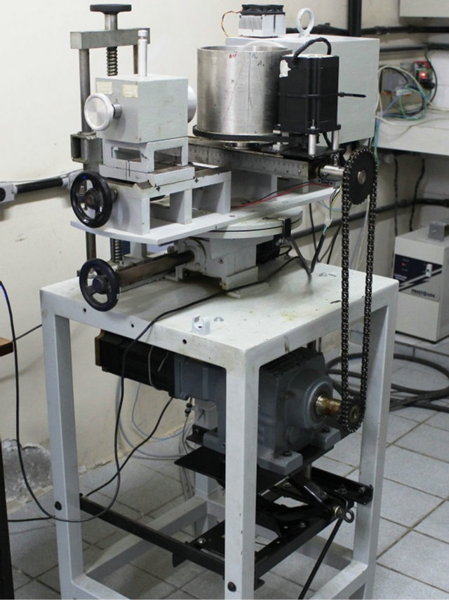
Figure 1. Gamma ray scanner.
defined according to gamma beam diameter Δs. In the experiments, a pure aluminum half-moon, well defined shape with 12.0 cm length and 6.0 cm radius was used as test object.
2.2. Tomography Parameters
By scanning an object the number of the gamma rays trajectories and the beam diameter choice: involve temporal, spatial and density resolutions as they are closely correlated parameters. For a third generation tomography process spatial resolution is strongly linked to the collimation of detectors, the number of detectors per projection and the number of projections. A question of measurement resolutions to time (speed of response), matter (e.g. density which defines the contrast in each pixel) and space (spatial resolution which defines how detailed the image is), as given in reference [1]. In single beam tomography, temporal resolution takes into account the number of projections needed for generating one image. Evaluation of parameters and their interaction quantification, certainly, are required in the tomography process, even if no standard proceedings are established for caring out parameters determination. Contrary to medical XRay CT a universal method, in Gamma Ray CT each group construct herself scanner to investigate the Industrial process and, define specific parameters methodology. The tomography parameters resolutions of density, spatial and temporal, were carried out for the scanner hardware used in this work and methodology is described in [6]. Linearity is an additional parameter which is required as one fundamental Equation (3) computes a liner function. The surface area integration, of the object all along rotation angles measured in tomography experiment, keeps a constant value within expected errors, as the experiment demonstrate the linearity property of the scanner and their uncertainty also was estimated [7].
The main sources of errors in tomography process are: 1) Contribution of measurement system;
2) Geometric magnification factor;
3) Tomography reconstruction algorithms.
They are well accepted in literature, and for the FCCFluidized Catalytic Cracking process the irradiation geometry of the riser a stainless cylinder, tube wall effect is include as source of errors. Contribution of measurement system is given in [8], and geometric factor is considered in [9]. Tube wall effect was evaluated by means of a mathematical model developed to simulate attenuation and estimate errors [10]. Aiming industrial process tomography, reconstruction algorithms requiring reduced number of data were studied [11].
3. Data Analysis and Modeling
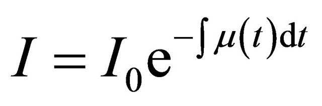
The mathematical fundaments in gamma ray tomography process are described by means of Beer-Lambert based equations, as
 (1)
(1)
 (2)
(2)
 (3)
(3)
 (4)
(4)
In Equation (1) the gamma intensities I, I0 with and without absorber are related to the linear attenuation coefficient μ, and x is the gamma ray path length. The Equations (2) gives the integration of the attenuation coefficient μ(t) at position t, and logarithm and discrete form of integral are the expressed in Equation (3). This Equation (3) is a usual form to generate matrix data for computational algorithm reconstruction. In Equation (4), the gamma intensities were adapted to riser irradiation geometry as IV, IF for empty tube and at flow conditions, related to the mass attenuation coefficient α. The riser internal diameter is D and on the left side ρm is mean density along gamma ray path.
The gamma beam width and sampling procedure for the gamma ray trajectories are following requirements to data analysis in scanning process [8], and measurement precision in actual experiment follows prescribed conditions.
Taken tomography row data several information are available prior to calculation of parameters given in Equations (1) to (4). In Figures 2 and 3 it can be observed the whole data points from the scanner process. They are two different stain tubes; the one from Figure 2 has less wall thickness than the tube in Figure 3, the aluminum half moon is in both of them. Object position at the tube cross-section should be precisely defined, and such pictures might be useful therefore. In Figure 3 object is centralized and it is not in the Figure 2. Centralized position produces a defined inversion band of high and low gamma intensity, precisely and reproducible. Contrary to non centralized position that makes a hole on the intensity. No farther understanding about it but object parameters calculation proves the visual information from Figures 2 and 3.
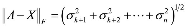
Attenuation coefficient is a prime parameter in all calculations given by Equations (1) to (4). Experimental and reconstructed data needs a metric to compare the approximation and RMSE-Root Mean Square Error is widely used for that evaluation. Appling for the row data, calculated with Equation (3) and comparing with attenuation coefficient from literature value [12], a precise approximation was obtained with the RMSE calculation, only for selected data points. Checking this calculation with the Frobenius norm, which is normalized for the ROI-region of interest, as it appears in the RMSE expression. The norm was checked by means of their singular values decomposition as
 (5)
(5)
where the two matrixes are, in this work, attenuation coefficient reference A and measured values X. For which difference the Frobenius norm is equal to the expression on the right side of Equation (5), according to known linear algebra theorem. Although the metric was applied correctly but RMSE value, estimation is depending of the ROI-region of interest. In this experiment a good approximation for mass attenuation was found by excluding extremes data. RMSE is recommended by [1], nevertheless, discussion and the need to compare with other metrics in several fields of work can be found [13]. In Tomography data RMSE is widely applied and also comparison with other metrics shows that a specific quantification of reconstruction quality is often required.
A further evaluation of attenuation coefficient measurement was carried out, taken the whole matrix acquisition data 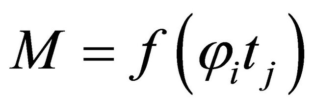 with i = 12 and t trajectories with j = 61. Experimental matrix was of M(12, 97) size, but the attenuation coefficient calculation takes just the object region M(12, 61). In this region, by collecting a vector of values from one angle φ from the data acquisition matrix M(1, 61) the μ evaluation was carried out. At first calculating μ given in Equation (3), for known object length and then the mean value of the vector data
Figure 2. Gamma ray profile of a steel tube and tomogramphy object.

Figure 3. Gamma intensity along tube and object region.
was obtained. Taken as reference mass attenuation coefficient α =  = 0.07802 cm2/g, and
  = (0.2098 ± 0.0004) cm−2, with density ρ = 2.7 g/cm3. The standard deviation of μ considers a statistical dispersion of 0.4% among the values given in literature [12] for X-ray mass attenuation coefficient and a negligible dispersion for the ρ value. For this vetctor a mean value of 0.1928 cm−1 was measured corresponding to an error of 8% error. The following step, takes the whole object region matrix M(12, 61), and again μ was calculated with the mean value of this matrix. This measure mean value μ = 0.2001 cm−1 is associated to a 5% error.
In addition, it might be considered that α literature values of aluminum are given for a long energy interval [12], in which 0.6 MeV is the nearest value for measuring with a 137Cs (0.662 Mev) radioactive source, therefore, approximation eror should also be taken into account. Then, a polonomial interpolation with sufficient reference values was carried out and a 0.0720 cm2/g value for mass attenuation coefficient of the 0.662 Mev photon, was found. Now, recalculating  with α = 0.0720 cm2/g value, the errors in measurig linear attenuation coefficient were of 0.8% in one vector and a 3% error for the whole matrix data. Attenuation coefficient evaluation in row data, as it is given in Figure 4, might provide a initial test for tomography transmission measurements By transmission measurements, Equations (1) to (4) will calculate just positive values, obviously, as there is no physical meaning for a negative value in such data. In Figure 5 is shown the test object experimental and calculated data with Equation (4). Considering that geometric center of the tube-riser coincides with the origin of coordinate system, by rotational scanning, data will be distributed on the four Cartesian quadrants. Therefore, to show the spatial distribution on a riser cross-section is necessary some data treatment. At first, carry out data rotation using a rotation matrix, to follow the physical scanner motion. Rotation matrix is applied for several data analysis techniques [14], and applying for the simulated data in Figure 6, spatial distribution of attenuation interval follows rotation angle φ form 00 to 1800. But, didn’t succeed for experimental data, due to a scanner motion blur on the test object shape. In order to obtain a spatial distribution of test object a further data treatment was required.
Attenuation interval should be explicit as it gives a measure of object suface by means of sufficient scanned
Figure 4. Linear attenuation coefficient versus length of aluminum half-moon.
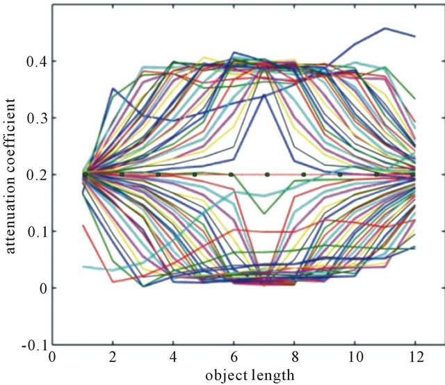
Figure 5. Linear attenuation coefficient versus object length for the acquisition matrix of measured data.
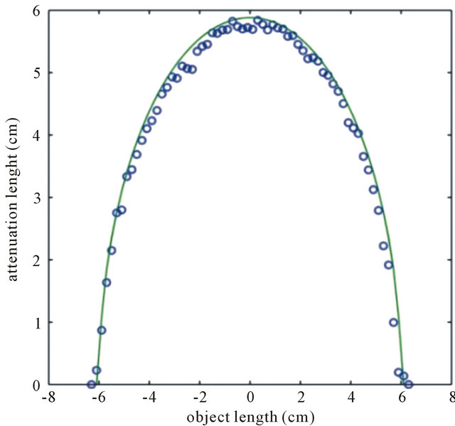
Figure 6. Attenuation interval measured in circles and calculated data in line.
data. By re-arranging Equation (4), in order to place length dimension on the left side as attenuation interval on the right side will remain object density ρ and α is mass attenuation coefficient as given in Equation (4).
Experimental aluminum half-moon data were used for evaluation of tomography process and to show spatial distribution. The model developed for simulate attenuation as a function of internal and external tube radii [10], was applied by using internal tube and object test radii. As it works well, next step the modeled data will undergo rotation by means of matrix rotation C calculated as
 (6)
(6)
where B is a vector of modeled data, ![]() are rotation errors and the answer is the A vector of modeled data at the measured angle φ. The result, experimental data of the test object at spatial distribution of test object, can be visualized in Figures 7 and 8.
are rotation errors and the answer is the A vector of modeled data at the measured angle φ. The result, experimental data of the test object at spatial distribution of test object, can be visualized in Figures 7 and 8.
4. Results and Discussion
Figure 2 shows row data obtained with the scanner given in Figure 1.
Whole scanning interval can be seen, in Figure 2, the I0 gamma intensity appears before and after steel tube. Two data sets are superposed empty tube and tube with object, IV, IF intensities for calculations with Equation (4). Superposition makes precision of the scanner operation easy to visualize.
In Figure 3 the scanning interval shows only the tube within object region.
Figure 4 shows linear attenuation coefficient measurement data, between green and red lines, representing mean within a 2σ confidence interval.
In Figure 4 can be seen the data points of the mean value μ = 0.1928 cm−1. Attenuation coefficient was determined also with measurement data in whole matrix as given in Figure 5. The line and points at the middle of the graph to show an attenuation coefficient value of μ = 0.2001 cm−1.
Object test, aluminum half moon mesured and calculated data, at zero angle φ, is seen in Figure 6.
Simulation of half-moon under scan rotation, fits object shape moving around origin of coordinete system, as Figure 7, shows it at one rotation angle φ.
To visualize experimental data tourning around origin of coodinate system scanned object data was modeled and then under matrix rotation as it is shown in Figures 8 and 9.
The same data procedure is given also in Figure 9 to
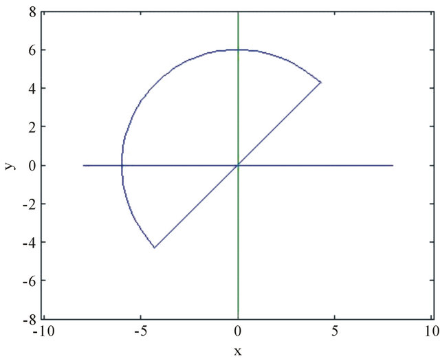
Figure 7. Attenuation length versus object length by simulated object at angle φ of 45˚.
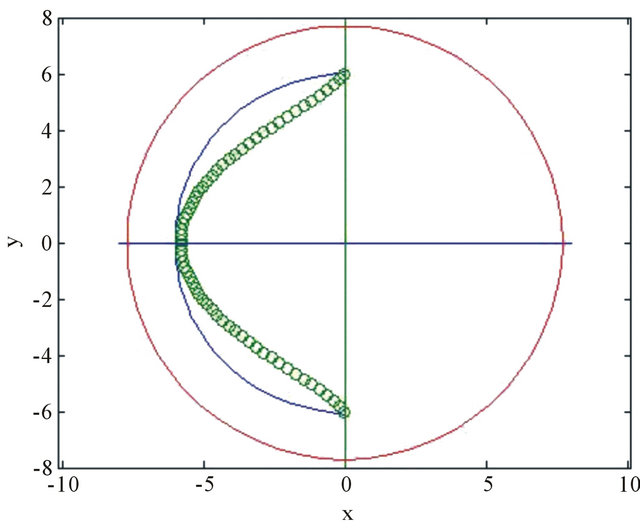
Figure 8. Experimental modeled data in circles, object shape and internal tube circumference in line at rotation angle φ of 90˚.

Figure 9. Experimental modeled data in circles, object shape and internal tube circumference in line at rotational φ of 120˚.
show object spatial distribution.
Spatial distribution in cross-section area is visualized inside internal tube diameter. Errors, due to modeling and matrix rotation calculation can be observed for departure from object shape in line, are of 11%. Comparing with Figure 6, for experimental and calculated data the corresponding errors are of 3%.
As industrial tomography reconstruction aims reduced number of data [11], and experiments brings erros to imaging process, information as scanner data generation shown in Figures 2 and 3, end precision evaluation as given in Figures 4 and 5, should be prior to any model validation. A simple evaluation as Figures 8 and 9, ilustrates the procedure that might provide useful information to industrial porcess prior and to compare with tomography reconstruction.
5. Conclusion
Attenuation coefficient is precisely measured in row data from tomography process. Space distribution is shown in attenuation length to compare with object shape, but surely, any other required parameter can be calculated and modeled. Analysis with row data is shown and it could be used for any matrix size at same conditions. The procedure is simple, effective and should be prior to any data treatment for opaque vessel reactor and by reconstruction algorithm in process imaging.
6. Acknowledgements
The authors are grateful to CNPq for the Scholarships and financial support and to Dr. Waldir Martignoni of Petrobrás for technical assistance.
REFERENCES
- IAEA-International Atomic Energy Agency, “Industrial Process Gamma Tomography,” IAEA-TECDOC-1589, 2007.
- M. Azzi, P. Turlier, J. R. Bernard and L. Garnero, “Mapping Solid Concentration in a Fluid Bed Using Gammametry,” Powder Technology, Vol. 67, No. 1, 1991, pp. 27-36. doi:10.1016/0032-5910(91)80023-C
- J. Gilby and J. Walton, “Data Visualization,” Software Support for Metrology Good Practice Guide No. 13, 2003.
- J. Sanyal, S. Zhang, G. Bhattacharya, P. Amburn and R. J. Moorhead, “A User Study to Compare Four Uncertainty Visualization Methods for 1D and 2D Datasets,” IEEE Transactions on Visualization and Computer Graphics, Vol. 15, No. 6, 2009, pp. 1209-1218.
- P. C. L. da Costa, C. C. Dantas, C. A. B. O. Lira and V. A. Dos Santos, “A Compton Filter to Improve Photopeak Intensity Evaluation in Gamma Ray Spectra,” Nuclear Instruments and Methods in Physics Research Section B, Vol. 226, No. 3, 2004, pp. 419-425. doi:10.1016/j.nimb.2004.05.037
- C. C. Dantas, S. B. Melo, E. F. Oliveira, F. P. M. Simões, M. G. dos Santos and V. A. dos Santos, “Measurement of Density Distribution of a Cracking Catalyst in Experimental Riser with a Sampling Procedure for Gamma Ray Tomography,” Nuclear Instruments and Methods in Physics Research Section B, Vol. 266, No. 5, 2008, pp. 841- 848. doi:10.1016/j.nimb.2008.01.029
- A. E. Moura, T. L. Rolim, C. C. Dantas, L. G. Charamba, D. A. Vasconcelos, S. B. Melo, V. A. dos Santos, E. F. Carvalho, J. A. C. Silva and R. Narain, “Gamma Ray Computer Aided Tomography of Adaptive Scanner System for Different Type and Size Columns,” IMEKO Metrology Congress—II CIMEC, Natal, 2011.
- C. C. Dantas, R. Narain, V. A. dos Santos and A. C. B. A. de Melo, “Catalyst Concentration Distribution in Fluidized Bed by Gamma-Ray Absorption,” Journal of Radioanalytical and Nuclear Chemistry, Vol. 269, No. 2, 2006, pp. 425-428. doi:10.1007/s10967-006-0402-4
- A. Aquino-Filho, C. C. Dantas, M. L. Crispino, E. A. O. Lima and V. A. Dos Santos, “A Gamma Ray Tomography Design for Catalyst Concentration Reconstruction in a FCC Type Riser,” International Nuclear Atlantic Conference, Santos, 2005.
- C. C. Dantas, V. A. dos Santos, A. C. B. A. Melo and R. Van Grieken, “Precise Gamma Ray Measurement of the Radial Distribution of a Cracking Catalyst at Diluted Concentrations in a Glass Riser,” Nuclear Instruments and Methods in Physics Research Section B, Vol. 251, No. 1, 2006, pp. 201-208. doi:10.1016/j.nimb.2006.05.009
- G. V. Vasconcelos, S. B. Melo, C. C. Dantas, I. Malta, R. Oliveira and E. F. Oliveira, “A Particle System Approach to Industrial Topographic Reconstruction,” Measurement Science and Technology, Vol. 22, 2011, Article ID: 104003.
- J. H. Hubbell and S. M. Seltzer, “Tables of X-Ray Mass Attenuation Coefficients,” Radiation and Biomolecular Physics Division, PML, NIST, 1996.
- K. Juda, “Modeling of the Air Pollution in the Cracow Area,” Atmospheric Environment, Vol. 20, No. 12, 1986, pp. 2449-2458.
- H. Wang, “Measures of Agreement for Rotation Matrices with Application to Vectorcardiography Data,” InternetWanghn Paper, Nonparcomp Report, 2008.