American Journal of Operations Research
Vol.07 No.01(2017), Article ID:73606,8 pages
10.4236/ajor.2017.71004
Efficient Frontier via Production Functions and Mechanization
Hideki Nakamura
Faculty of Economics, Osaka City University, Osaka, Japan

Copyright © 2017 by author and Scientific Research Publishing Inc.
This work is licensed under the Creative Commons Attribution International License (CC BY 4.0).
http://creativecommons.org/licenses/by/4.0/


Received: November 24, 2016; Accepted: January 16, 2017; Published: January 19, 2017
ABSTRACT
This study attempts to reconcile data envelopment analysis (DEA) with the production function approach in economics. We examine not only the inputs of capital and labor, but also the ranges of these inputs in production process steps, and endogenously derive a Leontief production function. The Leontief production functions shift northeasterly owing to mechanization, which is the replacement of labor inputs by capital inputs in some steps. Consequently, we describe the efficient frontier as the convex hull of the Leontief production functions. Furthermore, we consider the possibility of efficient production below the efficient frontier.
Keywords:
Production Process Steps, Leontief Production Function, Mechanization, Efficient Frontier, Production below the Efficient Frontier

1. Introduction
When we explore production efficiency in economics using data envelopment analysis (DEA), we encounter two difficulties. The first difficulty is the impossibility of direct application of concave production functions. In DEA, the representation of an efficient frontier is as the convex hull of efficient production. However, we usually assume neoclassical production functions in economics. The second difficulty is the interpretation of production inside the efficient frontier. Unless production is located on the efficient frontier, it is difficult to consider efficient production.
This paper attempts to overcome these two difficulties by considering mechanization in production, a distinguishing feature of modern economic growth.1 We make two important assumptions. The first is that goods and services are produced through a process involving numerous steps and we differentiate between these steps based on whether labor or capital predominates.2 A firm then chooses the ranges of capital and labor in order to minimize production costs. Mechanization, which means the replacement of labor by machines, can be represented as an increase in the range of capital use, that is, a decrease in the range of labor use. The second assumption is that production extracts the minimum input among the inputs of steps, making it possible to consider a production bottleneck in the short run.
We derive endogenously the Leontief production function, in which the coefficients of capital and labor depend on the range of capital use, that is, the degree of mechanization. When the replacement of labor by machines saves costs because of an increase in the wage/interest rate ratio, firms adopt mechanization. The Leontief production function slides northeasterly as a result of mechanization. We can describe the efficient frontier using the convex hull of Leontief production functions. Because the production of a firm depends on its own efficiency of capital and labor use, given production of differentiated goods, we can then consider efficient production, even when below the efficient frontier.3
The study relates to two lines of research. The first is that the ranges of capital use and labor use in production make it possible to consider mechanization, which saves labor costs. Zeira [1] modeled mechanization and explored international differences in output per labor unit. Our study incorporates two important features in this regard. The first is that production extracts the minimum input among the inputs of steps, so we can endogenously derive the Leontief production function. The second is that we elucidate upon the process of mechanization which describes the transition from an old to a new mechanized technique.
The second line of research is the production frontier derived from mechanization. Examining complementary relationships between capital accumulation and mechanization, Nakamura and Nakamura (2008) [2] and Nakamura (2009) [3] derived constant-elasticity-of-substitution (CES) production functions. We derive the efficient frontier as the convex hull of Leontief production functions, making it possible to reconcile the production function approach in economics with DEA.
The remainder of the paper is organized as follows. We explore production in production process steps and derive the efficient frontier via Leontief production functions in Section 2. In Section 3, we examine production below the efficient frontier, and in Section 4, we conclude our paper with a brief summary.
2. Efficient Frontier via Production and Mechanization
We examine the production of goods and services via a production process that involves numerous steps. We consider the following production function, which extracts the minimum value among the steps:
(1)
where is the output at time and is the input of step at time .
We consider the division of the steps according to the input ranges of labor and capital. As shown in Figure 1, the range of capital use, which is represented by ( ), implies a continuum of production process steps in which capital is the input. Hence, the range of labor use represented by implies a continuum of production process steps for which labor is the input. It is possible to replace labor inputs by capital inputs from to ( ).
We assume perfect substitutability between the capital and labor inputs in each step:
(2)
where . We assume that and . and represent the efficient levels of capital and labor inputs for steps and , respectively. and are the capital and labor inputs in step at time , respectively.
A firm determines input quantities and mechanization in order to minimize production costs. The adoption of mechanization is equivalent to the choice of techniques between and .
Given , the input quantities must satisfy for any and ( and ) because of the Leontief-type steps in (1). Thus, we obtain:
(3)
Equation (3) implies the following relationship between the total inputs and the degree of mechanization:
(4)
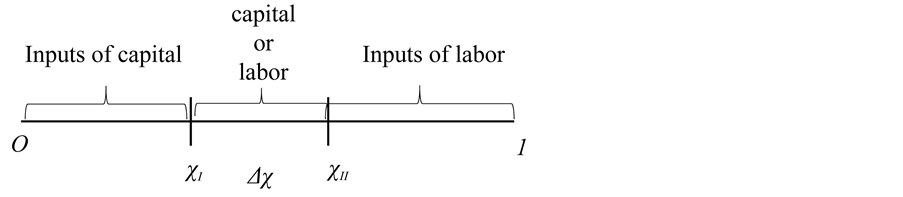
Figure 1. Input ranges of capital and labor in production process steps.
where and are the total inputs of capital and labor, respectively. and represent the total efficiency of capital and labor use, respectively:
We examine the properties of and . We obtain:
(5)
Equation (5) implies: and because and . Thus, in (4), holds. When the range of capital use increases, but that of labor use decreases, we have relatively fewer efficient steps for capital use and relatively more for labor use. Thus, the progress in mechanization requires an increase in the inputs ratio of capital to labor.
The degree of mechanization measured by the range of capital use implies an appropriate technique to combine capital and labor. Using (4), which describes the relationship between inputs and the degree of mechanization, we obtain the following Leontief production function, in which the coefficients depend on the degree of mechanization:
(6)
This implies:
where . is the output per labor unit and is capital
per labor unit.
We now explore mechanization as represented by the choice of technique between and . Given factor prices, the average cost minimization is as follows:
(7)
By rewriting , we define:
(8)
where . Note that and in (5) imply:
We consider the threshold in the ratio of the wage rate to the interest rate, in
which the two techniques, and , are equivalent: . We
obtain:
(9)
By comparing the production costs of and , firms decide whether to adopt the mechanization. Depending on factor prices, there are the following three cases. The first is a choice of technique χI when . It means no commencement of mechanization. Next, the use of technique is indifferent between and when . Because it makes no difference to firm profits whether they replace labor with machines, firms can commence mechanization. Finally, firms choose technique when . Firms adopt only the mechanized technique.
Depending on the degrees of mechanization, (4) implies the following input ratios of capital to labor:
(10)
Lemma 1: (Leontief production functions and mechanization). Given the assumptions in (1) and (2), the output per labor unit is represented as follows:
(11)
where represents the diffusion ratio using technique .
Proof: When , the capital and labor inputs are represented as follows, respectively:
where and ( ) are, respectively, capital and labor used in technique . We thus have:
where and represent the diffusion ratios using technique in capital and labor, respectively.
Dividing by while using the relationships between and , we obtain:
where ( ). The diffusion ratio using technique increases
with : , in which and .
Figure 2 describes the production functions in equilibrium with the two thresholds, and . When , we have the Leontief production function, represented as , in which the optimal output/capital ratio and output per capita are represented as and , respectively. When , mechanization begins. The Leontief production function slides northeasterly, which is represented as in the periods of . Depending on the capital/labor ratio of a firm, the firm gradually adopts the new mechanized technique. The process of mechanization, which shows the transition from the old technique, , to the new mechanized technique, , appears on the line between and . Finally, when , we have the Leontief production function, represented as , in which the optimal output/capital ratio and output per capita are represented as and , respectively.
Proposition 1: (Efficient frontier via production and mechanization). Given the assumptions in (1) and (2), the Leontief production functions are endogenously derived while the production functions shift northeasterly with mechanization. Consequently, the efficient frontier is represented as the convex hull of Leontief production functions.
In Figure 2, we can show the efficient frontier using the lines, , , , and . Given , production with a small is represented on the line between and . Given , production with a small is represented on the line between and .
Finally, we examine increases in the efficiency of capital and labor use.4
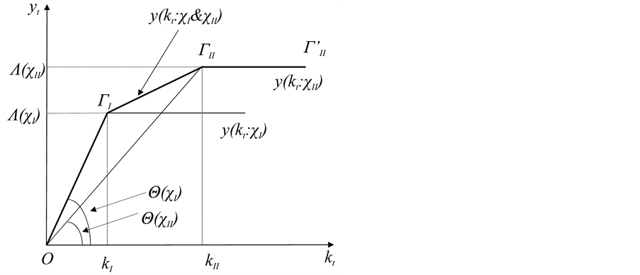
Figure 2. Efficient frontier via production and mechanization.
Increases in the efficiency of capital and labor use are capital- and labor-aug- menting technical progress, respectively. Given the degree of mechanization, represented as , capital-augmenting technical progress increases the slope of the Leontief production function, represented as an increase in . An increase in promotes mechanization. Labor-augmenting technical progress increases the efficient frontier, represented as an increase in with an increase in the capital/labor ratio. An increase in retards mechanization.
3. Production below the Efficient Frontier
We now explore what production below the efficient frontier means. We presume the following production functions of firms and :
(12)
where and . and are assumed to be differentiated goods. For simplicity, the ranges of capital use, and , are equal for the two firms, and .
We assume that both the aggregate efficiencies of capital and labor use are lower for firm than for firm :
(13)
Given (13), the efficient frontier is formed by firm . The production and mechanization of firm are represented below the frontier (see Figure 3). Depending on and ( , ), firms have different timings of mechanization. If a relative decrease in the aggregate capital use to aggregate labor use is smaller for firm than for firm , firm can have mechanization first, even when it is below the frontier.
Finally, we mention the possibility of leapfrogging. If firm can have a further mechanization with ( ), it is possible for firm to leapfrog, that is, to form the new frontier (see Figure 3).
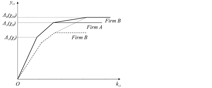
Figure 3. Efficient production and mechanization of firms and .
Proposition 2: (Region below the efficient frontier). We consider production of differentiated goods. When the aggregate efficiencies of capital and labor use are both lower than those of the efficient frontier, production is represented below the frontier. However, firms can have efficient production and mechanization that depend on their own efficiencies of capital and labor use.
4. Concluding Remarks
This paper attempted to reconcile DEA with the production function approach in economics. We considered the ranges of capital and labor use and endogenously derived a Leontief production function. We examined mechanization, as represented by the replacement of the labor input in some steps with capital input. Thus, we can describe the efficient frontier using the convex hull of Leontief production functions. Furthermore, we can explain the efficient production of firms below the frontier.
Cite this paper
Nakamura, H. (2017) Efficient Frontier via Production Functions and Mechanization. American Journal of Operations Research, 7, 56-63. http://dx.doi.org/10.4236/ajor.2017.71004
References
- 1. Zeira, J. (1998) Workers, Machines, and Economic Growth. Quarterly Journal of Economics, 113, 1091-1117. https://doi.org/10.1162/003355398555847
- 2. Nakamura, H. and Nakamura, M. (2008) A Note on the Constant-Elasticity-of-Substitution. Macroeconomic Dynamics, 12, 694-701. https://doi.org/10.1017/S1365100508070302
- 3. Nakamura, H. (2009) Micro {Foundation for a Constant-Elasticity-of-Substitution Production Function through Mechanization. Journal of Macroeconomics, 31, 464-472. https://doi.org/10.1016/j.jmacro.2008.09.006
NOTES
1We readily observe a high degree of mechanization in manufacturing industries. For example, labor used to be extensively used for most steps in producing clothing, but nowadays almost all of these steps are done by machines. Furthermore, robots with artificial intelligence can replace manual labor. It is now possible to have mechanization in service industries.
2When workers use machines, it should be possible to decompose their work into at least some steps.
3The efficiency of a firm depends on some factors which include the firm size and the type of differentiated goods and services, even in the same industry. Thus, it could be different among firms how capital and labor are efficiently used.
4The improvement of machines can increase the efficiency of capital use, . A more user- friendly technique can increase the efficiency of labor use, . Additionally, if a new technology creates some jobs, the input efficiency will change with the normalization of the number of steps.