

American Journal of Operations Research
Vol.06 No.06(2016), Article ID:72035,18 pages
10.4236/ajor.2016.66042
Explicit Exact Solution of Damage Probability for Multiple Weapons against a Unitary Target
Hongyun Wang1, Cardy Moten2, Morris Driels3, Don Grundel4, Hong Zhou5*
1Department of Applied Mathematics and Statistics, University of California, Santa Cruz, CA, USA
2TRADOC Analysis Center, Naval Postgraduate School, Monterey, CA, USA
3MAE Department, Naval Postgraduate School, Monterey, CA, USA
4Armament Directorate, Eglin AFB, Valparaiso, FL, USA
5Department of Applied Mathematics, Naval Postgraduate School, Monterey, CA, USA

Copyright © 2016 by authors and Scientific Research Publishing Inc.
This work is licensed under the Creative Commons Attribution International License (CC BY 4.0).
http://creativecommons.org/licenses/by/4.0/



Received: April 18, 2016; Accepted: November 13, 2016; Published: November 16, 2016
ABSTRACT
We study the damage probability when M weapons are used against a unitary target. We use the Carleton damage function to model the distribution of damage probability caused by each weapon. The deviation of the impact point from the aimpoint is attributed to both the dependent error and independent errors. The dependent error is one random variable affecting M weapons the same way while independent errors are associated with individual weapons and are independent of each other. We consider the case where the dependent error is significant, non-negligible relative to independent errors. We first derive an explicit exact solution for the damage probability caused by M weapons for any M. Based on the exact solution, we find the optimal aimpoint distribution of M weapons to maximize the damage probability in several cases where the aimpoint distribution is constrained geometrically with a few free parameters, including uniform distributions around a circle or around an ellipse. Then, we perform unconstrained optimization to obtain the overall optimal aimpoint distribution and the overall maximum damage probability, which is carried out for different values of M, up to 20 weapons. Finally, we derive a phenomenological approximate expression for the damage probability vs. M, the number of weapons, for the parameters studied here.
Keywords:
Damage Probability, Carleton Damage Function, Multiple Weapons with Dependent Errors, Exact Solution, Optimal Distribution of Aimpoint

1. Introduction
The probability of killing or damaging a target depends heavily on how close a weapon is delivered to the target. This delivery accuracy of a weapon may be affected by many components. In general, the errors are usually divided into two main groups: the dependent error and independent errors. The dependent error is related to the aiming error that results from a miscalculation of latitude, longitude, distance, wind effect, or uncertainty in locating the target position. The dependent error results in the armament impacting away from the desired target point and it affects all weapons the same way. The independent errors refer to ballistic dispersion errors, which may result from variations in bullet shape, variations in gun barrels, or variations in amount of explosive used inside each bullet [1] .
Due to many uncertainties in the field of weapon effectiveness, Monte Carlo simulations have been widely employed to estimate the probability of target damage [2] . Even though Monte Carlo simulations can provide reasonable estimates, exact solutions are mathematically more attractive and practically more useful. The objectives of this paper are: i) to derive explicit exact solution for the damage probability caused by multiple weapons against a single target, ii) to use the exact solution to maximize the damage probability with respect to the aimpoint distribution of weapons, with or without geometric constraint(s) on the aimpoint distribution, and iii) to study the relation of damage probability to the number of weapons when the dependent error is significant. The results obtained here can be applied to indirect fire artillery, or GPS/INS-guided weapons.
The remainder of this paper will progress as follows. Section 2 provides the detailed mathematical formulation and explicit exact solution for the kill probability. Section 3 considers the performances of various aimpoint distributions. Finally, Section 4 presents conclusions and future work.
2. Mathematical Formulation
We consider a single point target in the two dimensional space. We establish the coordinate system such that the target is located at the origin point . We use M weapons with dependent and independent errors to fire on the target. Due to the presence of significant dependent error, if all M weapons are aimed at
 , the M impact points may be uniformly shifted away from the target by a significant distance, resulting in a small damage probability. To make the damage probability less susceptible to the dependent error, we aim the M weapons at M different points distributed around the target. When the dependent error shifts some impact points away from the target, it simultaneously shifts the some other impact points toward the target. In this study all weapons are assumed to be perfectly reliable. Gross errors due to anomalies such as catastrophic weapon system failure, adverse weapon separation effects, and GPS jamming are neglected.
Let
・  = the aiming point of weapon j.
・  = miss distance from the aimpoint due to the dependent error of M weapons, affecting the impact points of all M weapons uniformly.
・  = miss distance from the aimpoint due to the independent error of weapon j, affecting only the impact point of weapon j individually. We assume that
  are independent of each other and independent of random variable
 .
.
The impact point of weapon j is given by

We model the dependent error  as a normal random variable with zero mean:

where  and
and  are standard deviations, respectively, in the two coordinate directions, which give an indication of the spread of the dependent error in the two directions. We model each independent error
  as a normal random variable with zero mean:

Further, we assume that the independent errors of individual weapons  are independent of each other and are independent of the dependent error
 .
.
We use the mathematical fact that the sum of two independent normal random variables is a normal random variable. Suppose  and
and . We have
 (1)
(1)
The probability density functions of U and V are given by


In terms of the probability density functions, we write Equation (1) as

Applying a change of variables , denoting
  still by u for simplicity and multiplying the equation by
 , we get

We rewrite the equation above in terms of expected values:
 (2)
(2)
Here the notation  indicates the average with respect to random variable U while z and
  are fixed, not varying with U. Equation (2) is valid for any normal random variable
 , and for any z and
 . In the analysis below, we will use Equation (2) extensively.
We use the Carleton damage function to model the probability of killing by an individual weapon. Let  be the impact point of a weapon where
  and
and  describe the impact points in the range and deflection directions from the target. The probability of the target being killed by a weapon at impact point
  is modeled mathematically as
 (3)
(3)
This is called the Carleton damage function or the diffuse Gaussian damage function [3] . The two parameters  and
and  in the Carleton damage function (3) represent the effective weapon radii in the range and deflection directions, respectively. With the impact points of the M weapons given by
 , the probability of the target located at the origin being killed by the M weapons is
 (4)
(4)
We calculate the probability of the target being killed averaged over independent errors  and averaged over the dependent error
 . For that purpose, we only need to calculate the average of each term inside the summation:
  . Notice that
  involves only the horizontal components and
  involves only the vertical components of
  and
and . Since the horizontal components and vertical components are independent of each other, we have

Since  and
and  have exactly the same format, we only need to derive the analytical expression for one. For conciseness, we denote
 ,
,  , and
, and  simply by
 ,
,  , and
, and  in the calculation of
 . We first average
  over independent errors
 .
.
 (5)
(5)
Each term in the product is an average of the form on the left hand side of (2). Applying Equation (2), we write each average as

Substituting this result into Equation (5), we obtain

Next we average over the dependent error . Again, the average is of the form on the left hand side of (2). Applying Equation (2), we arrive at

Thus, the overall average of  has the expression
 (6)
(6)
Similarly, the overall average of  has the expression
 (7)
(7)
The probability of target being killed, averaged over independent errors and dependent error, is called kill probability, and is denoted by . It has the expression
 (8)
(8)
where  and
and  are given in (6) and (7) above. Together, Equations (6)-(8), give us an explicit analytical expression for calculating the kill probability.
After the completion of the above derivation, we discovered that similar approaches had been taken separately by von Neumann [4] and by Washburn [5] .
3. Performances of Various Aimpoint Distributions of Multiple Weapons against a Single Target
Now we apply the exact solution to examine the kill probability corresponding to various distributions of the aimpoints of M weapons.
Let  denote the weapon lethal area or the fragmentation mean area of the effectiveness. It describes the effect of a warhead against a target and includes the effects of direct hit, blast, and fragmentation. We can calculate
  from the Carleton damage function (3) as
 (9)
(9)
The aspect ratio of the weapon radii of the Carleton damage function  is described by the empirical formula:
 (10)
(10)
where  is the impact angle.
Once the lethal area  and the aspect ratio a are given, one can calculate the weapon radii for the Carleton damage function (3) as follows:
 (11)
(11)
 (12)
(12)
For all the cases considered in this paper, we choose ,
, . This yields
  and
and . Furthermore, we choose
  for the dependent error and
  for the independent errors.
We first consider the case of M weapons with aimpoints uniformly distributed on a circle as formulated below

where r is the radius and  the phase off-set angle of the distribution. These are parameters that we can tune to maximize the kill probability.
For each value of M, we maximize the kill probability with respect to . This unconstrained nonlinear optimization can be achieved by using MATLAB built-in function fminsearch which is based on a direct search method of Lagarias et al. [6] . The results are listed in Table 1.
Note that the Carleton damage function we use is not isotropic. It has different effective radii in the range and deflection directions. To accommodate this anisotropic property of the Carleton damage function, we consider the case of M weapons with aimpoints distributed on an ellipse as formulated below

where  is the aspect ratio of the ellipse. In the formulation above, we elongate one axis by
  and simultaneously shrink the other axis by the same factor. In this way, the area of the ellipse is maintained at
 , independent of the aspect ratio
 . Parameter
  has the meaning

From  and
and , we can determine the major axis and the minor axis as
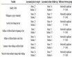
Table 1. The optimal distribution for M aimpoints when they are uniformly distributed around a circle and the corresponding probability of kill. Here r is the radius and q is the phase off-set angle.
The asterisks reflect that when r = 0, θ is not meaningful, meaning that θ is arbitrary and irrelevant.


We should point out that parameter  is not the polar angle of the aimpoint of weapon 1.
  is the angular value used in the parametric equation of the ellipse to calculate the aimpoint of weapon 1.
  is the phase angle before the major axis is elongated and before the minor axis is shrunk.
For each value of M, we maximize the kill probability with respect to . We obtain the results in Table 2.
In the above, we calculated the performance of placing the aimpoints of M weapons along a circle or an ellipse. We now examine the case of aiming one weapon at the center and aiming the rest  weapons at positions distributed on an ellipse. The aimpoints of M weapons are distributed as formulated below.


For each value of M, we maximize the kill probability with respect to . The optimal results are reported in Table 3.
Next, we fully optimize the distribution of M aimpoints without constraining them
Table 2. The optimal distribution for M aimpoints when they are uniformly distributed around an ellipse and the corresponding probability of kill. Here  is the off-set value in the parametric equation of the ellipse. The cases of
  and
and  are not affected by aspect ratio.
The asterisks reflect that when r = 0, θ is not meaningful, meaning that θ is arbitrary and irrelevant.
Table 3. The optimal distribution for M aimpoints when one of them is aimed at the origin while the rest of aimpoints are uniformly distributed around an ellipse, and the corresponding probability of kill. Here  is the off-set value in the parametric equation of the ellipse. For the cases of
 , the kill probability is not improved by moving one of the M aimpoints to the center.
When M = 1, there is only one aim-point at the center. The ellipse does not exist in this case. So the asterisks simply indicate that the values are irrelevant.
on a circle or an ellipse. We represent the M aimpoints in polar coordinates.

The optimal solutions for ,
,  ,
,  and
and  are listed in Table 4.
Figure 1 shows the optimal distributions of aimpoints for  (yellow circles) and
  (blue squares) while the optimal distributions for the cases of
  (yellow circles) and
  (blue squares) are displayed in Figure 2.
The optimal solutions for ,
,  ,
,  and
and  are given in Table 5.
Figure 3 illustrates the optimal distributions of aimpoints for  (yellow circles) and
  (blue squares); Figure 4 shows the optimal distributions of aimpoints for
  (yellow circles) and
  (blue squares).
Table 4. Optimal distributions of aimpoints and the corresponding probabilities of kill for ,
,  ,
,  and
and .
.

Figure 1. Optimal distributions of aimpoints for  (yellow circles) and
  (blue squares).

Figure 2. Optimal distributions of aimpoints for  (yellow circles) and
  (blue squares).
Table 5. Optimal distributions of aimpoints and the corresponding probabilities of kill for ,
,  ,
,  and
and .
.
The optimal solutions for ,
,  ,
,  and
and  are listed in Table 6.
Figure 5 displays the optimal distributions of aimpoints for  (yellow circles) and
  (blue squares); the optimal distributions for
  (yellow circles) and
  (blue squares) are plotted in Figure 6.
As M (the number of weapons) increases, the optimal distribution of aimpoints has more layers, covering a larger area with a more uniform distribution over the area. In Figure 7, we plot the optimal distributions of aimpoints for  (yellow circles) and
  (blue squares).
Next, we study the optimal kill probability as a function of M. Let  denote the kill probability corresponding to the optimal distribution of aimpoints for the case of M weapons. As M increases, the survival probability of the target,
  , decreases. In the absence of dependent error and when the aimpoints are all fixed at one point, the outcome of each weapon affected by its independent error is statistically independent of the outcome of other weapons affected by their own independent errors. In this situation, the probability of surviving M weapons is simply the M-th power of the probability of surviving one weapon:
 . In other words, in the absence of dependent error, the log survival probability is a linear function of M.

Figure 3. Optimal distributions of aimpoints for  (yellow circles) and
  (blue squares).

Figure 4. Optimal distributions of aimpoints for  (yellow circles) and
  (blue squares).
Table 6. Optimal distributions of aimpoints and the corresponding probabilities of kill for ,
,  ,
,  and
and .
.

Figure 5. Optimal distributions of aimpoints for  (yellow circles) and
  (blue squares).

In the presence of dependent error, however, the situation is completely different. The same dependent error affects all M weapons. The outcomes of individual weapons are no longer independent of each other. As a matter of fact, when the M weapons are all aimed at the same position, the outcomes of individual weapons are highly correlated with each other. As an example, we examine the case of aiming all M weapons at the origin. The averages of  and
and  are calculated from Equations (6) and (7) as


The kill probability is

Figure 6. Optimal distributions of aimpoints for  (yellow circles) and
  (blue squares).

Figure 7. Optimal distributions of aimpoints for  (yellow circles) and
  (blue squares).

In the absence of dependent error, we have , and the kill probability is

In the presence of dependent error, to simplify the analysis, we assume that the independent errors are zero  and assume that
 . The kill probability becomes

For the first few values of M, we obtain


Using mathematical induction, we can prove that

Clearly, when all M weapons are aimed at the same positon,  decays less than geometrically with M.
With the optimal distribution of aimpoints for M weapons, we may expect that  decays faster than in the case of aiming all M weapons at the same position. Indeed, as demonstrated in the left panel of Figure 8, when the M weapons are aimed according to the optimal distribution of aimpoints,
  decays much faster than in the case of aiming all M weapons at
 . The right panel of Figure 8 shows the enhancement in the decay of survival probability
  attributed to the optimal distribution of aimpoints. Specifically, in the right panel of Figure 8, we plot the quantity below as a function of M

Even with the optimal distribution of aimpoints, however, the log survival probability,  , does not decrease linearly with respect to M in the presence of dependent error. In the left panel of Figure 9, we plot
  vs. M. It is clear that in the presence of dependent error, the survival probability decreases slower than the geometric decay.
After excluding the geometric decay, we explore the possibility of a power law decay for the survival probability. Specifically we examine whether or not the survival probability obeys the power law . If the survival probability follows this power law relation, then the plot of
  vs.
vs.  would be a linear function

In the right panel of Figure 9, we plot  vs.
vs. . The plot demon-

Figure 8. Left panel: Comparison in the decay of survival probability , of the case of aiming all M weapons at
  vs. the case of using optimal distribution of aimpoints. Right panel: Enhancement in the decay of survival probability
  attributed to optimizing the distribution of M aimpoints.

Figure 9. Left panel: plot of  vs. M. Right panel: plot of
  vs.
vs. .
.

Figure 10. Left panel: plot of  vs.
vs. . Right panel: plot of
  vs. M.
strates clearly that the survival probability does not follow a power law decay.
To find a phenomenological fitting to the decay of survival probability as a function of M, we consider the form of . If the survival probability approximately satisfies this relation, then the plot of
  vs.
vs.  would approximately follow a straight line.

In the left panel of Figure 10, we plot  vs.
vs. . The plot is very close to a straight line. In the right panel of Figure 10, we plot
  vs. M and the fitting function
 . For the set of parameter values used, phenomenologically we have the approximation:

4. Conclusion
We have considered the damage probability caused by multiple weapons against a single target. Explicit exact solution was derived for the damage probability in the case of M weapons with both dependent error and independent errors. Then we applied the explicit exact solution to maximize the damage probability and find the corresponding optimal distribution of aimpoints. We observed that in the presence of significant dependent error, the decay of the survival probability corresponding to the optimal aimpoints distribution (i.e., 1 - optimal damage probability) is slower than the exponential decay with respect to M, the number of weapons. This observation demonstrates that increasing M is much less effective in overcoming the dependent error than in overcoming independent errors. We find that phenomenologically the survival probability decays exponentially with respect to a fractional power of M. Presumably, the fraction power varies with the parameter values of the problem. The mathematics behind this phenomenological expression and the dependence of the fraction power on the parameter values will be investigated in future studies.
Disclaimer
H. Zhou would like to thank TRAC-M for supporting this work. The views expressed in this document are those of the authors and do not reflect the official policy or position of the Department of Defense or the U.S. Government.
Cite this paper
Wang, H.Y., Moten, C., Driels, M., Grundel, D. and Zhou, H. (2016) Explicit Exact Solution of Damage Probability for Multiple Weapons against a Unitary Target. American Journal of Operations Research, 6, 450-467. http://dx.doi.org/10.4236/ajor.2016.66042
References
- 1. Driels, M. (2014) Weaponeering: Conventional Weapon System Effectiveness. 2nd Edition, American Institute of Aeronautics and Astronautics (AIAA) Education Series, Reston.
- 2. Chusilp, P., Charubhun, W. and Koanantachai, P. (2014) Monte Carlo Simulations of Weapon Effectiveness Using Pk Matrix and Carleton Damage Function. International Journal of Applied Physics and Mathematics, 4, 280-285.
http://dx.doi.org/10.7763/IJAPM.2014.V4.299 - 3. Washburn, A. and Kress, M. (2009) Combat Modeling. Springer, Dordrecht and New York.
http://dx.doi.org/10.1007/978-1-4419-0790-5 - 4. von Neumann, J. (1941) Optimimum Aiming at an Imperfectly Located Target, Appendix to Optimum Spacing of Bombs or Shots in the Presence of Systematic Errors. Ballistic Research Laboratory, Report 241.
- 5. Washburn, A. (2003) Diffuse Gaussian Multiple-Shot Patterns. Military Operations Research, 8, 59-64.
http://dx.doi.org/10.5711/morj.8.3.59 - 6. Lagarias, J.C., Reeds, J.A., Wright, M.H. and Wright, P.E. (1998) Convergence Properties of the Nelder-Mead Simplex Method in Low Dimensions. SIAM Journal of Optimization, 9, 112-147.
http://dx.doi.org/10.1137/S1052623496303470