American Journal of Operations Research
Vol.4 No.3(2014), Article ID:45682,10 pages DOI:10.4236/ajor.2014.43013
Optimal Stopping Time to Buy an Asset When Growth Rate Is a Two-State Markov Chain
Pham Van Khanh
Military Technical Academy, Hanoi, Vietnam
Email: van_khanh1178@yahoo.com
Copyright © 2014 by author and Scientific Research Publishing Inc.
This work is licensed under the Creative Commons Attribution International License (CC BY).
http://creativecommons.org/licenses/by/4.0/


Received 13 March 2014; revised 13 April 2014; accepted 20 April 2014
ABSTRACT
In this paper we consider the problem of determining the optimal time to buy an asset in a position of an uptrend or downtrend in the financial market and currency market as well as other markets. Asset price is modeled as a geometric Brownian motion with drift being a two-state Markov chain. Based on observations of asset prices, investors want to detect the change points of price trends as accurately as possible, so that they can make the decision to buy. Using filtering techniques and stochastic analysis, we will develop the optimal boundary at which investors implement their decisions when the posterior probability process reaches a certain threshold.
Keywords:Optimal Stopping Time, Posterior Probability, Threshold

1. Introduction
In [1] , the authors consider the problem of determining the optimal time to sell a property while price growth rate is a random variable that takes the value of the given set. Under the assumptions of the problem considered in [1] , growth rate only gets one of the possible values that do not change from this value to other values, which means that transition probability density is 0; but at a time I do not know the accuracy of price growth rate and the probability of receiving a certain value of growth rate also changes over time.
The authors in [2] also have much optimal stopping time in mathematical finance, but this is the classical problem and less common in practice because of its assumptions.
The authors in [3] consider the optimal stopping time problem when the growth rate of price process is not a random variable but in many cases.
In [4] the authors consider the problem to find the optimal time to sell when the price growth rate is Markov chain, however their approach is different from our method in this paper and the results are also different.
In this paper we consider the price process is described by geometric Brownian motion when its drift (price growth) is the Markov chain with two states 0 and 1 (0: decrease, downtrend; 1: increase, uptrend).
There is a phenomenon known as the momentum of the stock price, which means that the stock price has increased or is increasing, it will be increased in the future (usually near future), and a stock price has decreased or is decreasing, it will be decreased in the future. The investment is based on the momentum of price process that is called the momentum trading or trend following trading. By this way if an investor holding an asset wants to sell the asset, he will have to wait until a bull appeared and continues to hold such assets to the next price increase (in momentum) and when momentum is no longer available, i.e. prices going down or just starting going down, then he decides to sell. Similarly, if a person wants to buy an asset, he will wait for the appearance of an opportunity of going down in price and wait for prices to go down further (in momentum) until no longer falling price, then he decides to buy. According to this way of investment, investors are expected to buy the property at the bottom of market and sell the property at the highest point of the market.
In this paper, we analyze how to select buy and sell optimal strategies for a momentum trading. More precisely, we seek to maximize the expected profit from a momentum trade.
The method we use to study in this paper is the martingale theory, change of measure and the optimal stopping time is referred in the literature [2] [5] and [6] .
2. Buying Asset Problem
Now we consider the case , is a Markov chain with two states 0 and 1 that
 and only capable of moving from state 0 to state 1 with transition density as follows
At the time of ![]() we put
we put  where
where  is the filter generated by X.
We now consider the problem: Find ![]() -stopping time
-stopping time  such that:
 (2.1)
(2.1)
According to the theorem 9.1 (view [5] ), posterior probability process ![]() satisfying:
satisfying:

where

and  is a Brownian motion and the filter generated by
  coincides with filter
![]() .
.
Thus the process  satisfies the equation:

Then the process  and the posterior probability process
 ![]() satisfies the equation:
satisfies the equation:
 (2.2)
(2.2)
Put . According to Ito formula we have:

Definition process  as follows:
![]()
And the new measure  satisfying:

where .
.
According to Girsanov theorem,  is a
is a  -Brownian motion.
We have:


Consider the following process:

Is a ![]() -martingale and
-martingale and  with
with 
Let  is process determined by
 , we have
Consider the following process:
 According to Ito formula we have:

From this we have  (a.s.), then
 .
.
Denote  then
then 
Problem (2.1) is equivalent to the following problem:
 (2.3)
(2.3)
Put . According to Ito formula we have:
So, the drift of  is
is , it will be positive if
 , and it will be negative if
 . This suggests to us that the optimal stopping time is the first time the process hits
  in area
  with some A. Moreover pair
  satisfy the following free boundary problem:
 (2.4)
(2.4)
where ![]() is infinitesimal operator
is infinitesimal operator .
.
Differential Equation in (2.4) has the general solution as follows:

where


and


Changing variables and using some analytic transformations we obtain

and 
Denote
 .
.
We have

Now we consider the property of the function .
.
First, we calculate the derivative of .
.

Because  so
so .
.
According to average integral theorem we have 
where . Moreover, with small enough z we have
 . Then we have:
  when
when ![]() because
because ![]() and
and .
.
We have  because
  so
so

And then  is increasing function.
Moreover  because

So  and
and  means that the function
  is increasing and convex function on
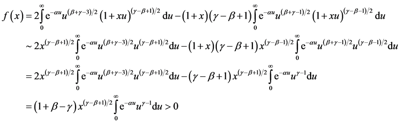
 . Figure 1 shows the graph of function
 , we can check the increase and convex properties of it. The graph of
  is shown in Figure 2, we can see that it tends to infinite when z as 0+.
But , then
  so
so 
By (2.4) we have 
So A is the solution of equation
 (2.5)
(2.5)
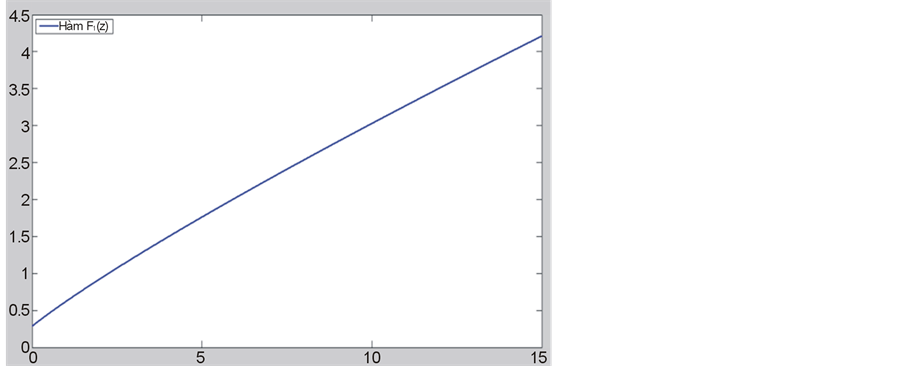
Figure 1. Graph of the function .
.
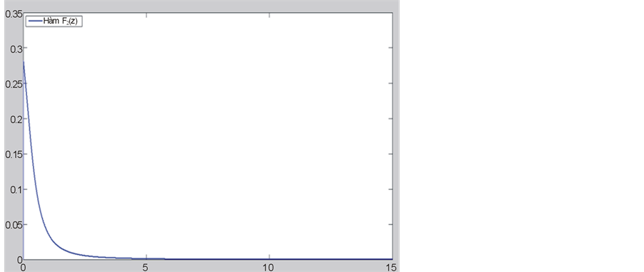
Figure 2. Graph of the function .
.
Lemma 2.1. Equation (2.5) has unique solution.
Proof: Equation (2.5) is equivalent to

Put: 
We have 
For integrals

So: 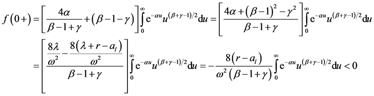

Because

and so 
We will prove 
Indeed, for large enough x we have ![]() and
and
Thus,  và
và is increasing function so
  have unique experience. So the theorem is proved.
The graph of  is shown in Figure 3, it is an increase function and
 .
.
Theorem 2.2. Stopping time  is the optimal stopping time for (2.1).
Proof:
According to the general theory of optimal stopping time is the point of making the expression:

is positive will be under the continuation area: .
.
And stopping time will be optimal if it is the first time that the ![]() hits the stopping regions
hits the stopping regions or
or .
. 
In Figure 4, we see a simulation of processes: Asset Price process, process , threshold probability, posterior probability process and the optimal stopping time with
 .
.
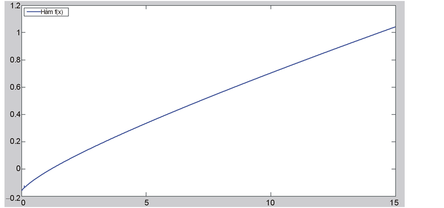
Figure 3. Graph of the function .
.
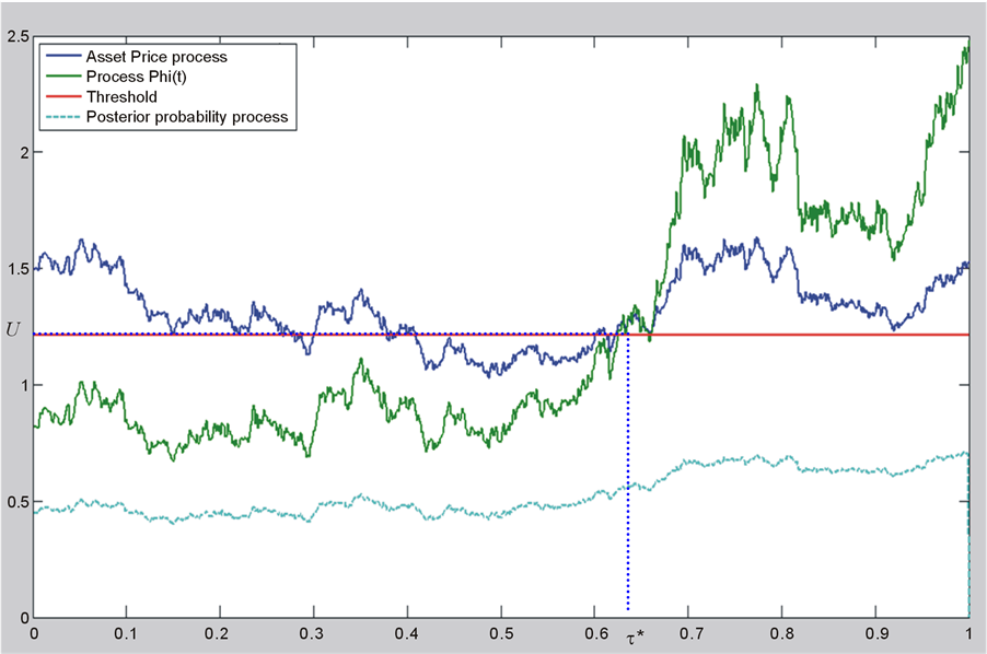
Figure 4. A simulation of asset price process, the posterior probability process, process , the threshold probability and the optimal stopping time (the optimal time to buy).
We find that  and the asset price (discounted) to buy is
 . In Figure 5, we simulate 4 processes: Asset Price process, process
 , threshold probability posterior probability process and the optimal stopping time with parameters
 .
.
We find that  and the asset price (discounted) to buy is
 .
.
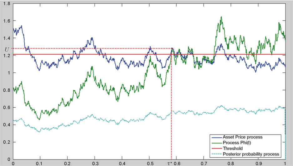
Figure 5. A simulation of asset price process, the posterior probability process, process , the threshold probability and the optimal stopping time (the optimal time to buy).
3. Conclusion
In this paper, we consider the problem of buying an asset when the asset price is modeled by the geometric Brownian motion which has a change point, where price growth rate is the Markov process with two states that describes the decreasing and increasing of asset prices process on the market. For buying problem we assume that the price will be a shift from decreasing to increasing prices and a buying decision is made when the probability of decreasing state surpassed some certain threshold. We have to simulate the price process with a number of parameters and conduct numerical solution to the experimental buying threshold. In the next study we will consider the problem with assumptions that are closer to reality and more constraints.
Acknowledgements
This research is funded by Vietnam National Foundation for Science and Technology Development (NAFOSTED) under grant number 10103-2012.17
References
- Khanh, P. (2012) Optimal Stopping Time for Holding an Asset. American Journal of Operations Research, 2, 527-535. http://dx.doi.org/10.4236/ajor.2012.24062
- Peskir, G. and Shiryaev, A.N. (2006) Optimal Stopping and Free-Boundary Problems (Lectures in Mathematics ETH Lectures in Mathematics. ETH Zürich (Closed). Birkhäuser, Basel.
- Shiryaev, A.N., Xu, Z. and Zhou, X.Y. (2008) Thou Shalt Buy and Hold. Quantitative Finance, 8, 765-776. http://dx.doi.org/10.1080/14697680802563732
- Guo, X. and Zhang, Q. (2005) Optimal Selling Rules in a Regime Switching Model. IEEE Transactions on Automatic Control, 50, 1450-1455.
- Lipster, R.S. and Shiryaev, A.N. (2001) Statistics of Random Process: I. General Theory. Springer-Verlag, Berlin, Heidelberg.
- Shiryaev, A.N. (1978, 2008) Optimal Stopping Rules. Springer Verlag, Berlin, Heidelberg.