Journal of Analytical Sciences, Methods and Instrumentation
Vol.2 No.3(2012), Article ID:23282,4 pages DOI:10.4236/jasmi.2012.23023
Eigensolution Variability of Asymmetric Damped Systems
![]()
1School of Mechanical and Electronic Engineering, Wuhan University of Technology, Wuhan, China; 2Department of Automobile Engineering, Henan Polytechnic, Zhengzhou, China.
Email: chenjian_em@sina.com
Received May 21st, 2012; revised June 18th, 2012; accepted June 30th, 2012
Keywords: Design Sensitivity Analysis; Asymmetric Damped Systems; Rotor Dynamic Model; Condition Number
ABSTRACT
The characterization of energy dissipation or damping in rotor dynamic model is of fundamental importance. Noise and vibration are not only uncomfortable to the users, but also may lead to fatigue, fracture and even failure. During the design process of asymmetric damped systems, it is often required to make changes in the design variables such that the design is optimal. This paper is aimed at developing computationally efficient numerical methods for parametric sensitivity analysis. The algebraic method considered here computes the eigenvector sensitivity by assembling the derivatives of eigenproblems and the additional constraints into an algebraic equation. The coefficient matrix may be ill-conditioned since the elements of it are not all of the same order of magnitude. In this study, a new algebraic method is presented to compute the eigensolution variability of asymmetric damped systems. Some weight constants are introduced such that the proposed method is well-conditioned. The method is very compact and highly efficient, and the numerical stability is also demonstrated. Moreover, several special cases can be presented based on the similar idea of the proposed method. Finally, two numerical examples show the validity of the proposed method.
1. Introduction
Eigensolution sensitivities have become an integral part of many engineering design methodologies including structural design optimization, reliability, dynamic model updating, structural health monitoring and many other applications. Although calculating eigenvalue sensitivity can be obtain in a straightforward way, computing eigenvector derivatives resides several challenges, such as the singularity problem and asymmetric damped systems. Eigensensitivity analysis has received much attention over the past four decades. Many methods are restricted to the systems with symmetric matrices. However, a number of engineering structures have asymmetric system matrices, for example, the study of rotor dynamic model, the behavior of structure in fluid and the aircraft flutter.
The modal method approximates the derivative of each eigenvector by expressing it as a linear combination of all the eigenvectors so that the eigenvector derivative could be carried out by calculating the linear combination coefficients. In 1968, Fox and Kapoor [1] first derived the expressions of the first-order derivatives of eigensolutions for undamped symmetric systems. Many authors [2-5] have extended Fox and Kapoor’s method to the more general asymmetric conservative systems. Adhikari and Friswell [6] extended the modal method to the first-order and second-order derivatives of the eigensolutions of asymmetric damped systems. To reduce the number of eigenvectors needed to compute the derivative of each eigenvector, Zeng [7] presented a modified modal method for the complex eigenvectors in symmetric damped systems. Later, Moon et al. [8] extended the modified modal method to general asymmetric damped systems. Wang [9] derived a modified modal method by using a residual static mode to approximate the contribution of unavailable high order modes.
Nelson [10] presented another efficient method to simplify the computation of the derivatives of eigenvectors for undamped systems. The main idea of Nelson’s method is to express the derivative of each eigenvector as a particular solution and a homogeneous solution. In contrast to the modal method, Nelson’s method requires only the interest eigenvector. Sutter et al. [11] pointed out Nelson’s method is more efficient than the modal method for the reason that the modal method needs all or most of the eigenvectors to find the derivative of each eigenvector. Later, Friswell and Adhikari [12] extended Nelson’s method to first-order eigenvector derivatives for symmetric and asymmetric damped systems. Recently, Guedria et al. [13] extended Nelson’s method to the second-order eigenvectors derivatives for symmetric and asymmetric damped systems.
Rudisill and Chu [14] investigated an algebraic method computed the eigensolution derivatives by solving a linear system of algebraic equations, but the coefficient matrix of the algebraic equation is asymmetric matrix. Lee et al. [15,16] developed the algebraic method with a symmetric coefficient matrix for first-order and secondorder equations of motion, respectively. Guedria et al. [17] extended the algebraic method to compute the derivatives of eigensolutions for general asymmetric damped systems. It has demonstrated that this method is computationally more efficient than Nelson’s method [13] and the modal method [6]. Later, Chouchane et al. [18] extended their method to the second-order derivatives of eigensolutions and pointed out their method can be extended to compute the higher order eigensolution derivatives. Recently, Xu et al. [19] and Li et al. [20] adopted new normalizations and developed efficient algebraic methods for the computation of eigensolution derivatives for asymmetric damped systems. However, solutions of the eigenvector derivatives computed by Xu’s method and Li’s method are different from that computed by the traditionally existing methods due to the new normalizetions. In contrast to Xu’s method and Li’s method, the eigenvector sensitivities computed by Guedria’s method are identity with those determined by Nelson’s method [13]. However, the algorithm of Guedria’s method is lengthy and complicated. In addition, the algebraic method [14-19] is proposed by assembling the derivatives of eigenproblems and the additional constraints into an algebraic equation. As a result, the coefficient matrix of the algebraic method may be ill-conditioned since the elements in the coefficient matrix may be not all of the same order of magnitude. One challenge frequently come up is whether or not to have other method is compact, efficient, and well-conditioned.
In this study, an equivalent form is proposed for the supplementary constraint, from which an efficient algebraic method is proposed to compute the derivatives of eigenvalues and associated eigenvectors of asymmetric damped systems. To reduce the condition number of the coefficient matrix, some weight constants are introduced. This method is simple, compact and numerically stable. Moreover, several special cases can be presented based on the similar idea of the proposed method.
The second section of this paper introduces basic theory of asymmetric damped systems. The third section proposes a sensitivity analysis method of asymmetric damped systems. The fourth section extends the proposed method to some special cases. And the next section presents two numerical examples to illustrate the validity of the proposed method.
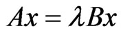
2. Basic Theory of Asymmetric Damped Systems
The second-order equation of motion describing the free vibration of a linear, damped discrete system with N DOF can be expressed as
 (1)
(1)
where M, C and K are, respectively, the mass, damping and stiffness matrices, t denotes time. Here the system matrices are asymmetric matrices and the mass matrix M is assumed to be a nonsingular matrix such that M–1 exists. q(t) represents the vector of generalized coordinates and has the exponential form
 (2)
(2)
Combining
and Equation (1) can easily obtain the equation of motion of 2N-space asymmetric damped systems
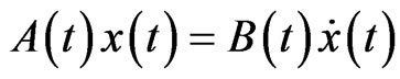 (3)
(3)
where

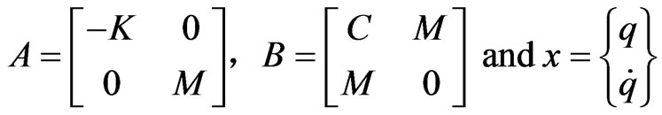 (4)
(4)
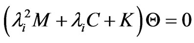
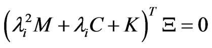
The right and left eigenproblem of a 2N-space asymmetric damped system can be represented, respectively, as follows:
 (5)
(5)
 (6)
(6)
where x and y are the right and left eigenvectors of 2N-space asymmetric damped systems.
For underdamped systems, the eigenvalues associated with Equations (5) and (6) appear in complex conjugate pairs
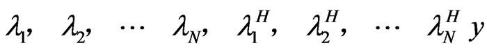
here  is the ith eigenvalue and
  denotes complex conjugate.
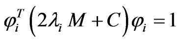
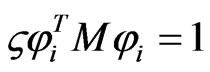
As the mass matrix is nonsingular, the right and left eigenvectors used to be normalized as the following form:
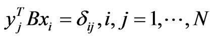 (7)
(7)
where  is the Kronecker delta,
  and
and  are the right and left eigenvectors corresponding to complex eigenvalue
 .
.
Substituting Equation (2) into Equation (1), the right eigenproblem of an N-space asymmetric damped system can be obtained
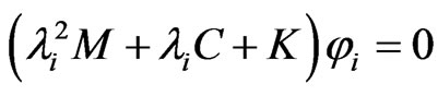 (8)
(8)
and the associated left eigenproblem is
 (9)
(9)
The eigenvectors between 2N-space asymmetric systems and N-space asymmetric systems satisfy
 (10)
(10)
Substituting Equation (10) into Equation (7), the normalization condition of an N space system can be obtained as following form:
It should be emphasized that the normalization condition expressed as Equation (11) is not sufficient to ensure uniqueness of eigenvectors for N-space systems, because when multiplying the left eigenvectors by any scalar and dividing the right eigenvectors by the same scalar, Equation (11) is also satisfied. Hence, an additional normalization condition should be imposed. In this paper,  denotes the eth component of the ith eigenvector. Many authors [6,13,17-21] adopted the additional normalization condition as follow
 (12)
(12)
which consists in setting one component in each pair left and right eigenvectors to be equal. That is to say, for the ith eigenvector pair, the eigenvectors are normalized so that the nith components are equal. The nith component is usually selected such that the product of the absolute values of the corresponding components in the eigenvectors is the largest. Thus
 (13)
(13)
3. Design Sensitivity Analysis Method
In this preceding section, an efficient algebraic method is presented to compute eigensensitivity. The eigensolutions of asymmetric damped systems are supposed to be known. The system matrices are assumed to depend continuously on the real design parameter p and their derivatives are known. For convenience, the following notation is adopted in this paper:
 .
.
3.1. The Singularity Problem
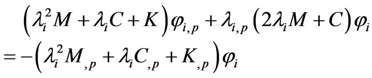
The differentiation of Equation (8) with respect to the design parameter p yields
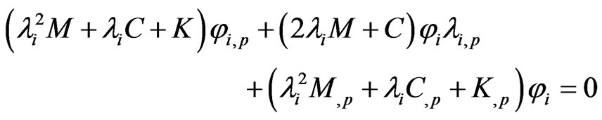 (14)
(14)
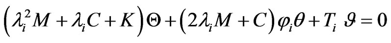
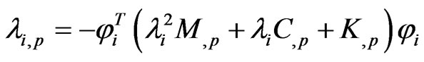
Premultiplying each side of the above equation by  and utilizing the normalization condition (11) and Equation (9), the eigenvalue derivatives can be obtained [12]
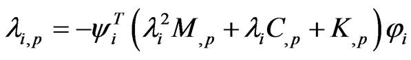 (15)
(15)
The derivative of eigenvalue given in Equation (15) only requires the corresponding eigenvalue and its associated left and right eigenvectors as well as the derivatives of system matrices. However, the derivatives of the right eigenvectors cannot be found directly utilizing Equation (14), because the coefficient matrix of the right eigenvector sensitivity is singular. The singularity is due to the fact that the rank of the matrix of order N is (N – 1) when the eigenvalues are distinct.
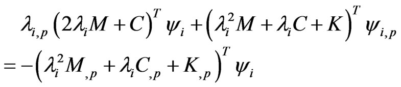
In a similar way, differentiating Equation (9) with respect to parameter p, the left eigenvectors derivatives satisfy
 (16)
(16)
For the same reason explained above, the derivatives of the left eigenvectors cannot be found directly using the above equation. Therefore, two additional constraints presented in the next subsection, should be imposed to uniquely determine the derivatives of the right and left eigenvectors.
3.2. Two Additional Constraints
To overcome the singularity problem, the existing methods usually use an additional constraint derived from the normalization condition by differentiating Equation (11) with respect to parameter p yields
 (17)
(17)
Note that the first right term of the above equation is a scalar, so we can obtain
 (18)
(18)
Hence, Equation (17) can be rewritten as
 (19)
(19)
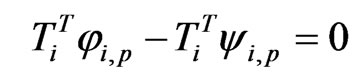
However, this above additional equation is not enough to uniquely determine the derivatives of the left and right eigenvectors. Therefore, a supplementary constraint should be imposed. Differentiating the new normalizetion condition expressed by Equation (12) with respect to the design parameter p, a new supplementary constraint can be obtain in the following form
 (20)
(20)
with
 (21)
(21)
 is a (N × 1) transform vector and the nith component of it associated with the ith left or right eigenvector is equal to 1. This expression means that the nith component of the ith right and left eigenvector derivatives are imposed to be equal.
3.3. The Proposed Method
In this subsection, a new method is proposed to compute simultaneously the derivatives of each eigenvalue and its associated left and right eigenvectors.
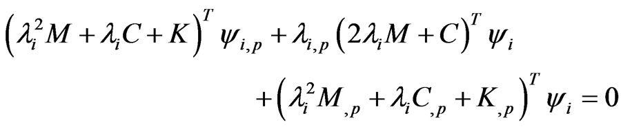
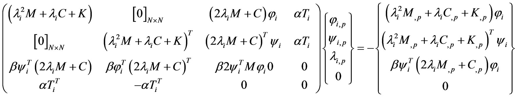
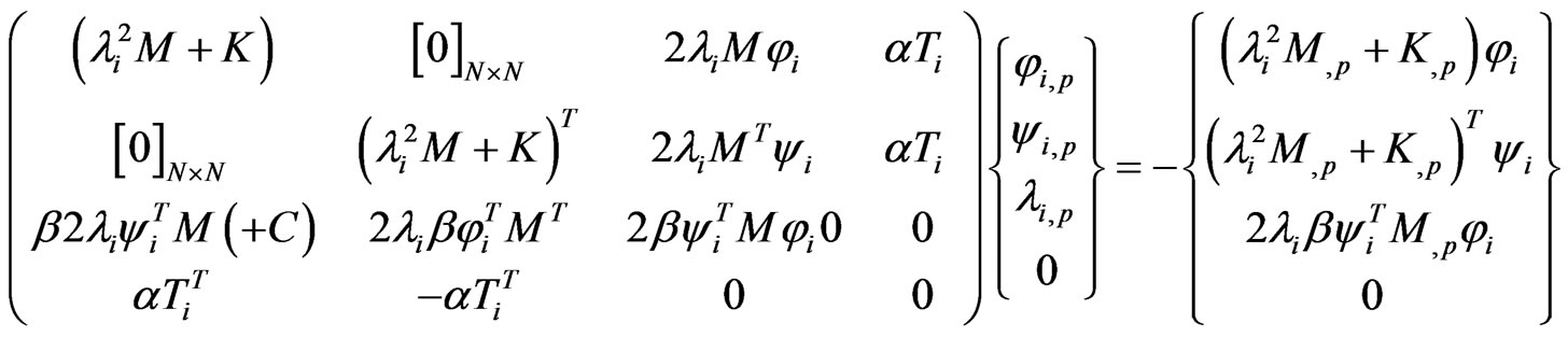
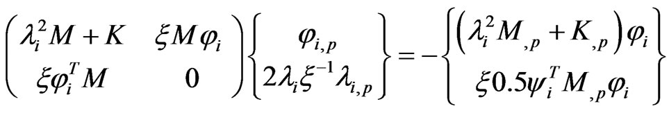
Rearranging Equations (14), (16), (19) and (20), respectively, as the follows forms:
 (22)
(22)
 (23)
(23)
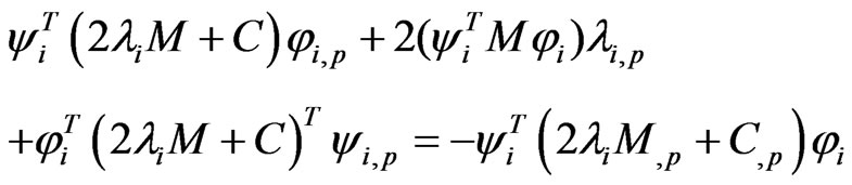 (24)
(24)
 (25)
(25)
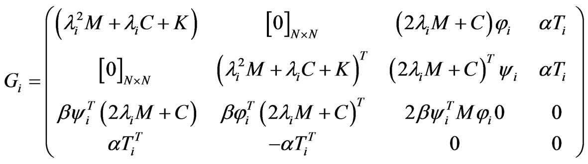
Rewriting the above four equations in the above algebraic matrix form (22)-(25).
α, β are weight constants. Because the equation is assembled by using the derivatives of eigenproblems and the additional constraints, the elements in the coefficient matrix may be not all of the same order of magnitude, as a result, the equation will has a large conditional number. To reduce the condition number, we select the non-zero constant β by
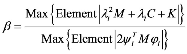
and select the non-zero constant α by
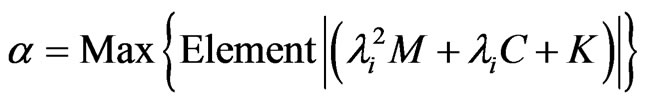
Substituting these weight constants into the above equation lead to a numerically well-conditioned system.
The Equations (26) constitute a linear system to obtain the eigensolution derivatives, and the system has the form
 (27)
(27)
with Gi a (2N + 2) × (2N + 2) coefficient matrix,  a (2N + 2) × 1 sensitivity vector and hi a (2N + 2) × 1 vector, which depend on eigensolutions and the derivatives of system matrices. The eigensolution sensitivities can be uniquely determined since the coefficient matrix Gi has a rank (2N + 2), as demonstrated in the following section.
The proposed method can be summarized as follows Step 1: Compute Gi and hi.
Step 2: Solve 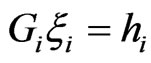 and obtain the eigensolution sensitivity.
Note that the algorithm of the proposed method contains only two steps, so it is very simple and compact.
3.4. Numerical Stability
In order to show that the coefficient matrix Gi of Equation (27) is nonsingular, consider a (2N + 2) × 1 vector, d and use the fact that the equation Gid = 0 has the unique solution d = 0.
Assume Gid = 0 with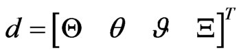 , i.e.,
 (29)
(29)
 (30)
(30)
 (26)
(26)
 (28)
(28)
 (31)
(31)
 (32)
(32)
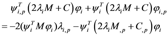
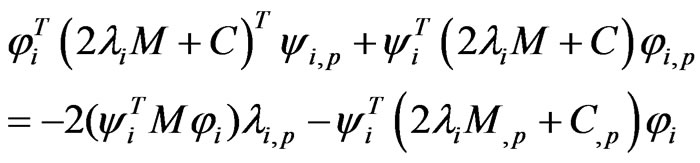
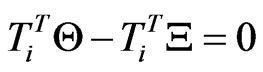
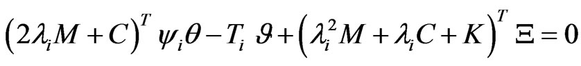
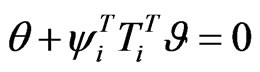
Premultiplying Equation (29) by  and premultiplying Equation (32) by
 , utilizing Equations (8), (9) and (11), thus
 (33)
(33)
 (34)
(34)
Combining the above two equations, one can obtain since
since . Substituting
 ,
,  into Equations (29) and (32), one can obtain
 (35)
(35)
 (36)
(36)
Comparing the above two equations with Equations (8) and (9), it is clear that  and
and  are particular solutions of Equations (35) and (36), respectively. Thus, solutions of the above two equations can be, respectively, expressed as
 (37)
(37)
 (38)
(38)
where  and
and  are constant coefficients. Substituting the above two equations and
  into Equations (30) and (31), respectively, and utilizing the additional normalization (11), one can obtain
 (39)
(39)
 (40)
(40)
Combining the above two equations, one can obtain . Due to the equation Gid = 0 has the unique solution d = 0, therefore, Gi is always a full rank matrix and the numerical stability of the proposed method can be guaranteed. As a consequence, the derivatives of eigensolutions can be uniquely determined utilizing Equation (27).
4. Special Cases
The proposed method can be extended to apply in several special cases. The following particular cases are considered: asymmetric undamped systems, symmetric damped systems and symmetric undamped systems. The derivatives of eigensolutions for the particular cases can be found by utilizing the similar procedure above.
4.1. The Asymmetric Undamped System
For asymmetric undamped systems, damp matrix is removed. The normalization condition (11) is reduced to

Considering the consistent normalization with traditional modal analysis for undamped systems,
is adopted as the normalization condition. With the similar idea of the proposed method, the algebraic system (26) can be simplified in the following form (41).
4.2. The Symmetric Damped System
For symmetric damped systems, the system matrices are all symmetric. The relation between the left and right eigenvectors and the derivatives of the right and left eigenvector are equal. Thus the normalization condition (11) can be simplified as
The new supplementary constraint expressed in Equation (20) will be ignored since it is always satisfied. Based on Equation (15), the eigenvalue sensitivity can be simplified as follow
 (43)
(43)
And, the algebraic system (26) can be reduced to the above form (43).
To reduce the condition number, selecting the nonzero constant  by
by
In the special case, when , the above equation is identical with that developed in [16], and Equation (43) may be considered as an development of the algebraic method [16].
 (41)
(41)
4.3. The Symmetric Undamped System
Assume the system matrices are all symmetric, and the damping matrix equals a zero matrix. Considering traditional mass normalization
The algebraic system (26) can be then reduced to the following form:
 (44)
(44)
where λi is the ith undamped natural frequency. Similarly, selecting the non-zero constant  by finding the absolute largest element of matrix
 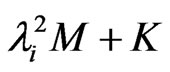 and dividing the largest element of
 . The above equation is similar with that developed in [15], and Equation (44) may be considered as a development of the algebraic method [15].
5. Numerical Examples
The validity of the proposed method will be demonstrated by the following two examples. The first example is a rotor dynamic model, which is used as an example of an asymmetric damped system. The second example is used to show the condition number of the improved algebraic method is remarkably reduced.
5.1. Example 1
To illustrate the application and efficiency of the proposed method, a rotor dynamic model, shown in Figure 1, is considered. The rotor dynamic model is an asymmetric damped system, which consists of a flexible shaft supported by two bearings and two rigid disks rigidly fixed to the shaft.
The shaft has a diameter d = 0.2 m, a length L = 5.0 m, a Young’s module E = 2.1 × 10¹¹ N/m2, a density ρ = 7850 kg/m3 and a Poisson’s ratio μ = 0.3. The disk1, fixed at L1 = 2.0 m from the left side of the shaft, has a 1.0 m external diameter and a 0.04 m thickness and the disk 2, fixed at L1 = 1.5 m from the right side of the shaft, has a 2.0 m external diameter and a 0.06 m thickness. The two bearings are identical and modeled using springs and dashpots with coefficients shown in Figure 1. The spring stiffness coefficients and the damping coefficients have the following values:
Kxx1 = Kxx2 = 5.2 × 10⁷, Kyy1 = Kyy2 = 3.2 × 10⁷ N/m and Cxx1 = Cyy1 = Cxx2 = Cyy2 = 1000 Ns/m.
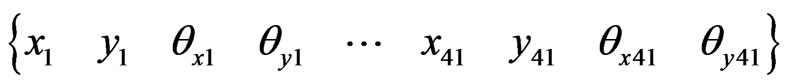
Bearing coefficients have been chosen such that the typical values of stiffness coefficients are used, with a slightly higher rigidity in the vertical direction [18], and moderate damping coefficients given in [6] are assumed. The rotor dynamic model is modeled using the finite element method. The rotor dynamic model is discretized into 40 shaft elements utilizing Timoshenko beam elements in which the gyroscopic effects are included. The coupling stiffness and damping coefficients of two bearing are assumed to be negligible. Each of the 40 elements has a length 0.125m and the system has 41 nodes. Each node has four degrees of freedom, the transverse displacements and the rotations in both the XZ plane and YZ plane. Hence, the model has 164 degrees of freedom, which are ordered as follows:
The two bearings are located at nodes 1 and 41, respectively. The disk1 is fixed at the 17th node and the disk 2 is fixed at the 29th node. The rotor dynamic model example is therefore a damped asymmetric model due tothe gyroscopic effects and the damping of the bearing dashpots.
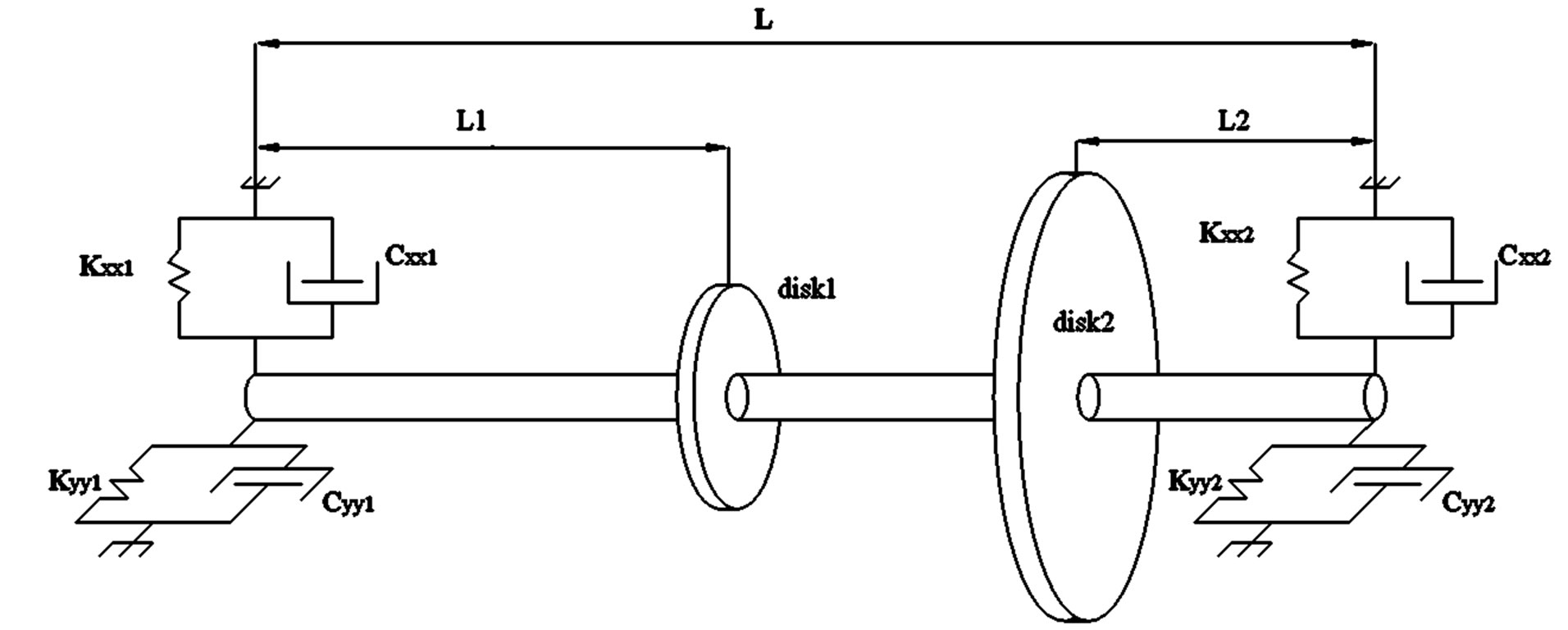
Figure 1. The geometric dimension and bearing model of the rotor dynamic model.
The Campbell diagram shown in Figure 2 depicts the change in the damped natural frequency with rotor speed. The system is numerically stable since the real parts of all eigenvalues are negative. The gyroscopic effects are significant leading to a five first critical speeds at 516, 540, 1620, 2268 and 2786 rpm, respectively. To illustrate the computation of the eigensolution derivatives using the proposed method, the operating speed of rotor dynamic model is chosen to be 2000 rpm. This speed is positioned between the third and the fourth critical speeds. In order to illustrate the computation of the eigensolution derivatives, the density of material has been chosen as a design parameter p. To compare solutions of the eigensolution sensitivities, eigensensitivities have been computed by Guedria’s method and the proposed method, respectively. Table 1 shows the first five eigenvalues and their derivatives. Tables 2 and 3 show some components of the first right and left eigenvectors, respectively. It has been checked that the eigenvector derivatives computed by the proposed method is the same results as that computed by Guedria’s method.
To illustrate the efficiency of the proposed method, the computational times of the eigensolution derivatives computed by the proposed method were compared with that obtained by Guedria’s method. Figure 3 shows the computational times of Guedria’s method and the proposed method with respect to the number of the computed eigensolution derivatives. The computation of the eigensolution derivatives have been repeated 10 times and the minimum and maximum times of the computation were removed, the average computational times are found to be 19.45 s for Guedria’s method and 14.38 s for the proposed method. To compute the derivative of each eigenpair, Guedria’s method needs multiply the reduced matrix of dimension ((2N +1) × 2N) for four times and requires solving a (2N + 1) linear equation, however, the proposed algorithm only needs solve a (2N + 2) algebraic equation.
A comparison of flop count is carried out next between Guedria’s method and the proposed method. The flop count is considered based on [20,22]. Let A and B be complex matrices of dimensions (m × n) and (n × p), respectively, the flop count of the product of A and B is (8 mnp - O(mp)). The Doolittle’s method computed a LU factorization Q = LU, costs 2n3 + O(n2) flops. Suppose that the first q eigensolution sensitivities. Here, the flop count for computing the eigensolutions and the derivatives of the system matrices is not considered. The total number of flops to implement the proposed method is [16N3 + O(N2)]q. And it is [16N3 + 128N3 + O(N2)]q for Guedria’s method (
 is sparsity parameter [21] which is unity for a full matrix). Therefore, the computational effort is reduced remarkably in contrast to Guedria’s method. In this special case, the computational time is
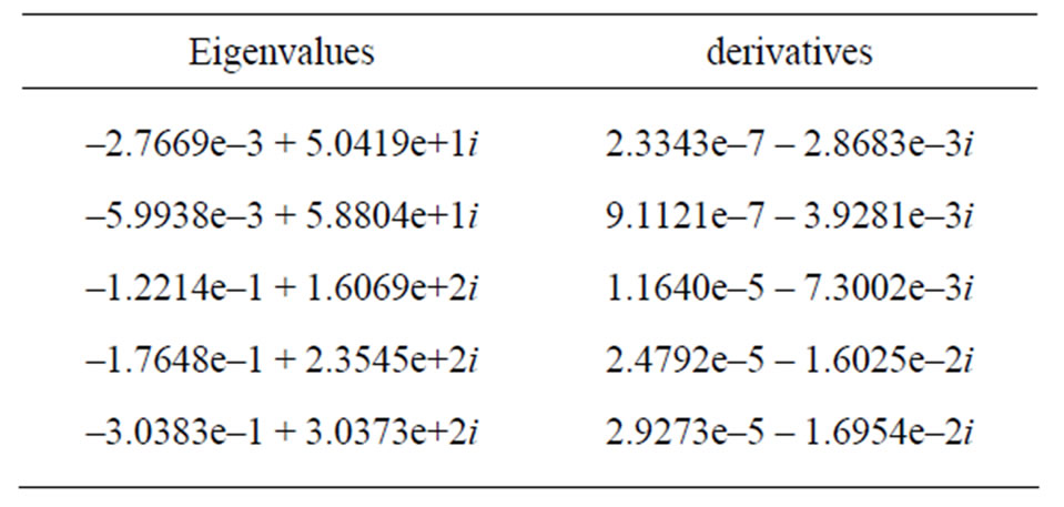
Table 1. The first five eigenvalues and their derivatives.
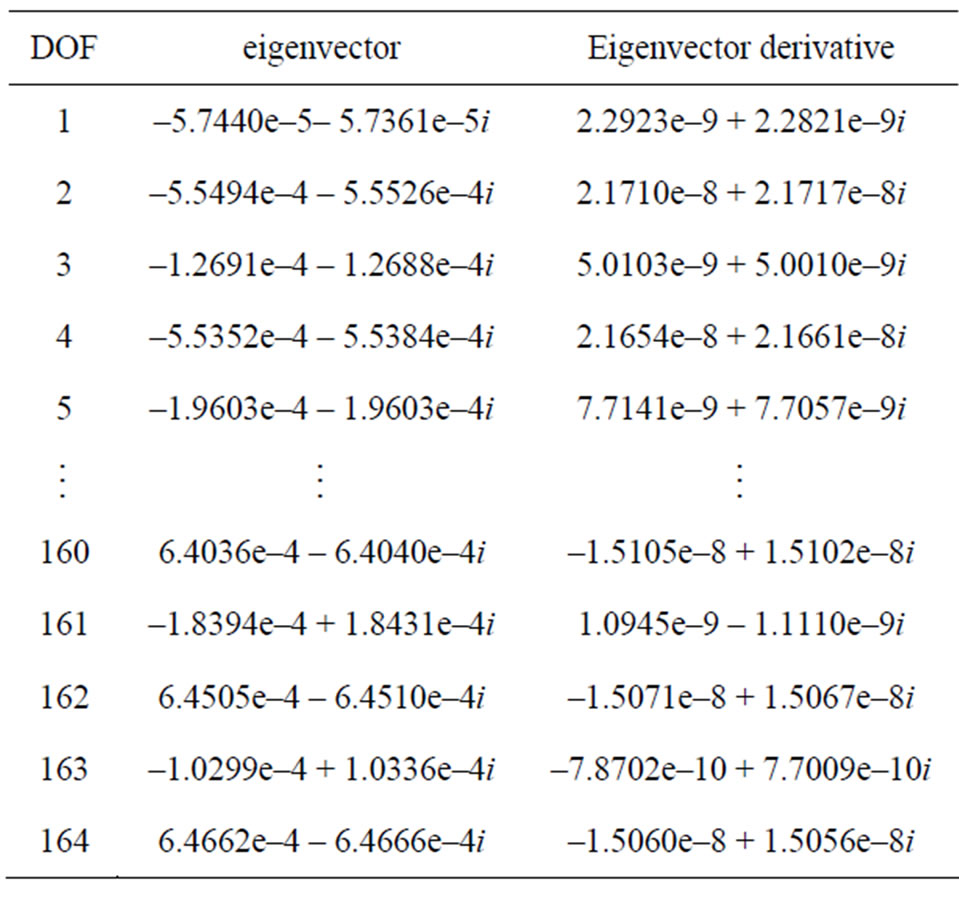
Table 2. The first right eigenvector and its first order derivatives.
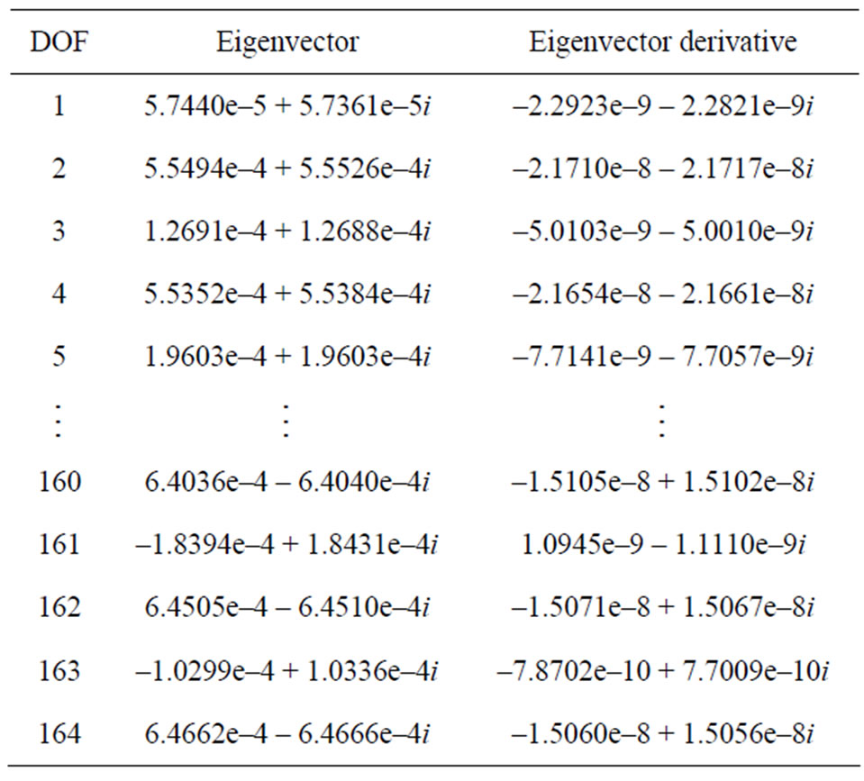
Table 3. The first left eigenvector and its first order derivatives.
reduced by about 26.1% in comparison with those elapsed by Guedria’s method. It has demonstrated that Guedria’s method is computationally more efficient than
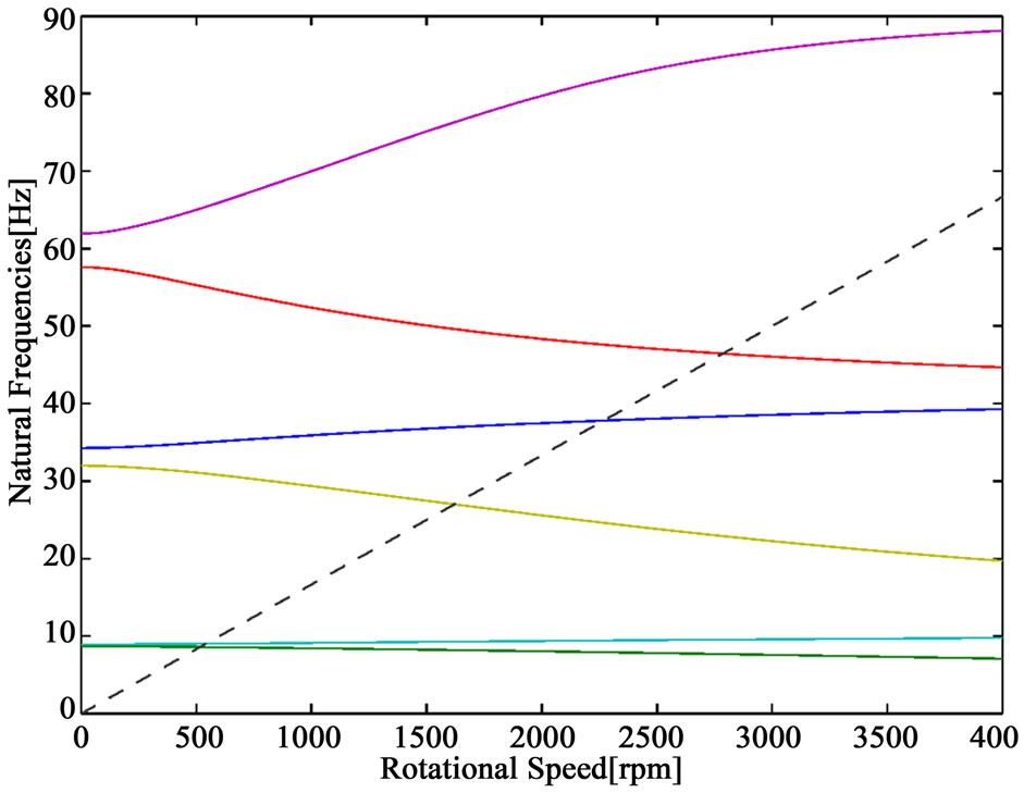
Figure 2. The Campbell diagram of the rotor dynamic model.
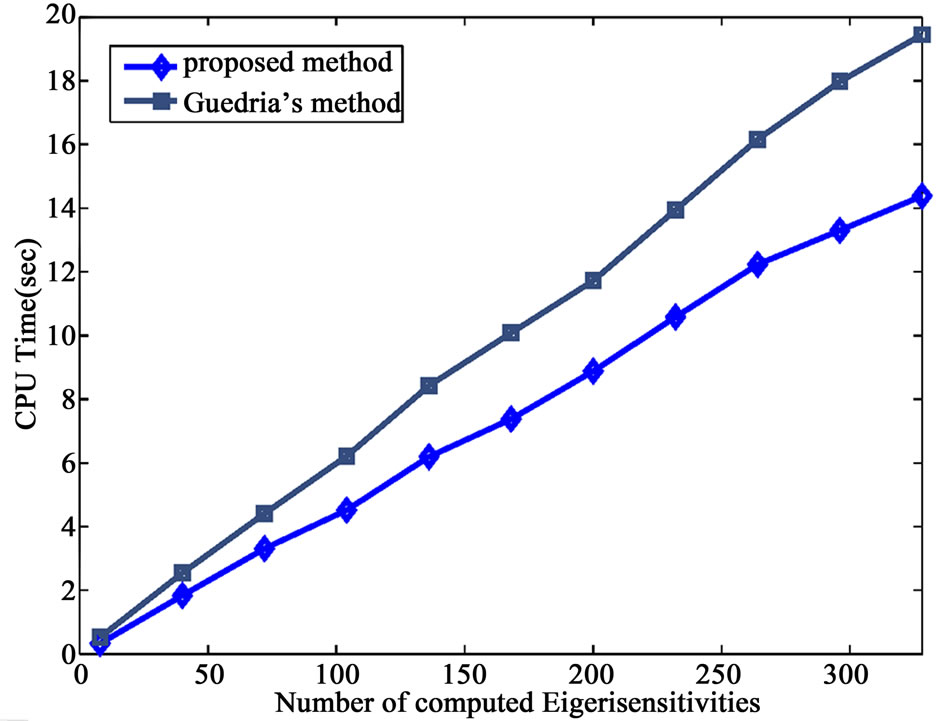
Figure 3. Comparison of CPU time.
Nelson’s method [12] and the modal method [6]. In this sense, it may be concluded that the proposed method is also computationally more efficient than both Nelson’s method and the modal method. Hence the proposed method gives exact eigensensitivity results and requires a lower computational cost.
5.2. Example 2
To illustrate the proposed method is well-conditioned, consider a 2-DOF mass-spring system. Assume the system matrices have the following form
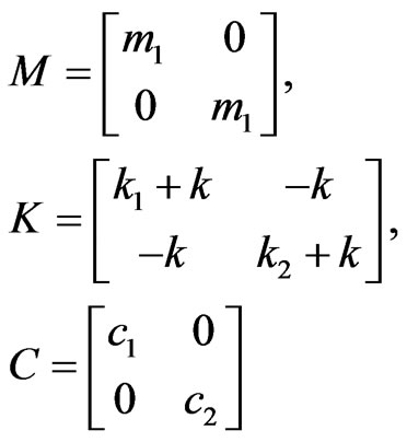
Suppose m1 = m2 = 1 kg, k1 = k2 = 10,000 N/m, c1 = c2 = 5.0 Ns/m. The stiffness k was chosen as the design parameter p, and the eigensolution derivatives were considered at k0 = 10,000 N/m. The system has two conjugate eigenvalues: –2.5 ± 99.969i and –2.5 ± 173.19i. The eigenvalue –2.5 + 31.524i was considered in this example. In this special case, the non-zero constant  is set to 1000.0 + 7.07i, the condition number of coefficient matrix is 7.07, and the condition number of the similar coefficient matrix in [16] is 1414.4. Therefore, the condition number is remarkably reduced, and the proposed method is numerically well-conditioned.
6. Conclusion
An improved algebraic method is presented for computing eigensolution derivatives of asymmetric damped systems with distinct eigenvalues. The method maintains N-space formulation without using 2N-space equations, and the proposed method is well-conditioned since elements of the coefficient matrix are all of the same order of magnitude. Several special cases can be presented based on the similar idea of the proposed method. This proposed method may be inserted easily into a comercial FEM code since it is very compact, numerically stable, and easy to be implemented on computers. When applying on a 164-DOF rotor dynamic model example, the computational time is reduced by about 26.1% in comparison with those elapsed by Guedria’s method [17]. And a two 2-DOF mass-spring system shows the condition number of the proposed method is reduced.
REFERENCES
- R. L. Fox and M. P. Kapoor, “Rates of Change of Eigenvalues and Eigenvectors,” AIAA Journal, Vol. 6, No. 12, 1968, pp. 2426-2429. doi:10.2514/3.5008
- L. C. Rogers, “Derivatives of Eigenvalues and Eigenvectors,” AIAA Journal, Vol. 11, No. 8, 1970, pp. 943-944. doi:10.2514/3.5795
- S. Garg, “Derivatives of Eigensolutions for a General Matrix,” AIAA Journal, Vol. 11, No. 8, 1973, pp. 1191- 1194. doi:10.2514/3.6892
- R. H. Plaut and K. Huseyin, “Derivative of Eigenvalues and Eigenvectors in Non-Self-Adjoint Systems,” AIAA Journal, Vol. 11, No. 2, 1973, pp. 250-251. doi:10.2514/3.6740
- C. S. Rudisill, “Derivatives of Eigenvalues and Eigenvectors for a General Matrix,” AIAA Journal, Vol. 12, No. 5, 1974, pp. 721-722. doi:10.2514/3.49330
- S. Adhikari and M. I. Friswell, “Eigenderivative Analysis of Asymmetric Non-Conservative Systems,” International Journal for Numerical Methods in Engineering, Vol. 51, No. 6, 2001, pp. 709-733. doi:10.1002/nme.186
- Q. H. Zeng, “Highly Accurate Modal Method for Calculating Eigenvector Derivative in Viscous Damping Systems,” AIAA Journal, Vol. 33, No. 4, 1995, pp. 746-751. doi:10.2514/3.12453
- Y. J. Moon, B. W. Kim, M. G. Ko and I. W. Lee, “Modified Modal Methods for Calculating Eigenpair Sensitivity of Asymmetric Damped System,” International Journal for Numerical Methods in Engineering, Vol. 60, No. 11, 2004, pp. 1847-1860. doi:10.1002/nme.1025
- B. P. Wang, “Improved Approximate Methods for Computing Eigenvector Derivatives in Structural Dynamics,” AIAA Journal, Vol. 29, No. 6, 1992, pp. 1018-1020.
- R. B. Nelson, “Simplified Calculation of Eigenvector Derivatives,” AIAA Journal, Vol. 14, No. 9, 1976, pp. 1201-1205. doi:10.2514/3.7211
- T. R. Sutter, C. J. Camarda, J. L. Walsh and H. M. Adelman, “Comparison of Several Methods for Calculating Vibration Mode Shape Derivatives,” AIAA Journal, Vol. 26, No. 12, 1989, pp. 1506-1511. doi:10.2514/3.10070
- M. I. Friswell and S. Adhikari, “Derivatives of Complex Eigenvectors Using Nelson’s Method,” AIAA Journal, Vol. 38, No. 12, 2000, pp. 2355-2357. doi:10.2514/2.907
- N. Guedria, M. Chouchane and H. Smaoui, “SecondOrder Eigensensitivity Analysis of Asymmetric Damped Systems Using Nelson’s Method,” Journal of Sound and Vibration, Vol. 300, No. 3-5, 2007, pp. 974-992. doi:10.1016/j.jsv.2006.09.003
- C. S. Rudisill and Y. Chu, “Numerical Methods for Evaluating the Derivatives of Eigenvalues and Eigenvectors,” AIAA Journal, Vol. 13, No. 6, 1975, pp. 834-837. doi:10.2514/3.60449
- I. W. Lee and G. H. Jung, “An Efficient Algebraic Method for the Computation of Natural Frequency and Mode Shape Sensitivities: Part I, Distinct Natural Frequencies,” Computers and Structures, Vol. 62, No. 3, 1997, pp. 429-435. doi:10.1016/S0045-7949(96)00206-4
- I. W. Lee, D. O. Kim and G. H. Jung, “Natural Frequency and Mode Shape Sensitivities of Damped Systems: Part I, Distinct Natural Frequencies,” Journal of Sound and Vibration, Vol. 223, No. 3, 1999, pp. 399-412. doi:10.1006/jsvi.1998.2129
- N. Guedria, H. Smaoui and M. Chouchane, “A Direct Algebraic Method for Eigensolution Sensitivity Computation of Damped Asymmetric Systems,” International Journal for Numerical Methods in Engineering, Vol. 68, No. 6, 2006, pp. 674-689. doi:10.1002/nme.1732
- M. Chouchane, N. Guedria and H. Smaoui, “Eigensensitivity Computation of Asymmetric Damped Systems Using an Algebraic Approach,” Mechanical System and Signal Processing, Vol. 21, No. 7, 2007, pp. 2761-2776. doi:10.1002/nme.1732
- Z. H. Xu, H. X. Zhong, X. W. Zhu and B. S. Wu, “An Efficient Algebraic Method for Computing Eigensolution Sensitivity of Asymmetric Damped Systems,” Journal of Sound and Vibration, Vol. 327, No. 3-5, 2009, pp. 584- 592. doi:10.1016/j.jsv.2009.07.013
- L. Li, Y. Hu and X. Wang, “A Parallel Way for Computing Eigenvector Sensitivity of Asymmetric Damped Systems with Distinct and Repeated Eigenvalues,” Mechanical System and Signal Processing, Vol. 30, No. 7, 2012, pp. 61-67. doi:10.1016/j.ymssp.2012.01.008
- D. V. Murthy and R. T. Haftka, “Derivatives of Eigenvalues and Eigenvectors of a General Complex Matrix,” International Journal for Numerical Methods in Engineering, Vol. 26, No. 2, 1988, pp. 293-311. doi:10.1002/nme.1620260202
- N. J. Higham, “Accuracy and Stability of Numerical Algorithms,” 2nd Edition, Siam, Philadelphia, 2002. doi:10.1137/1.9780898718027