 Engineering, 2013, 5, 933-942 Published Online December 2013 (http://www.scirp.org/journal/eng) http://dx.doi.org/10.4236/eng.2013.512114 Open Access ENG Power Law Exponents for Vertical Velocity Distributions in Natural Rivers Hae-Eun Lee1, Chanjoo Lee2, Youg-Jeon Kim2, Ji-Sung Kim2*, Won Kim2 1Department of Computational Science and Engineering, Yonsei University, Seoul, South Korea 2Water Resources Research Department, Korea Institute of Construction Technology, Goyang, South Korea Email: *jisungk@kict.re.kr Received October 5, 2013; revised November 5, 2013; accepted November 12, 2013 Copyright © 2013 Hae-Eun Lee et al. This is an open access article distributed under the Creative Commons Attribution License, which permits unrestricted use, distribution, and reproduction in any medium, provided the original work is properly cited. ABSTRACT While log law is an equation theoretically derived fo r near-bed region, in most cases, power law has been researched by experimental methods. Thus, many consider it as an empirical equation and fixed power law exponents such as 1/6 and 1/7 are generally applied. However, exponent of power law is an index representing bed resistance related with relative roughness and furthermore influences the shapes of vertical velocity distribution. The purpose of this study is to inves- tigate characteristics of vertical velocity distribution of the natural rivers by testing and optimizing previous methods used for determinatio n of power law exponen t with vertical velocity distribu tion data collected with ADCPs d uring the years of 2005 to 2009 from rivers in South Korea. Roughness coefficient has been calculated from the equation of Lim- erinos. And using theoretical and empirical formulae, and representing relationships between bed resistance and power law exponent, it has been evaluated whether the exponents suggested by these equations appropriately reproduce verti- cal velocity distribu tion of actual rivers. As a result, it has been confirmed that there is an incr easing tr end of pow er law exponent as bed resistance increases. Therefore, in order to correctly predict vertical velocity distribu tion in the natural rivers, it is necessary to use an exponent that reflects flow conditions at the field. Keywords: Vertical Velocity Distribution; Power Law Exponent; Natural Rivers; Field Measurement; Flow Resistance 1. Introduction In most cases, velocity profiles in wide open channels are expressed by either log law or power law. These laws are widely used not because they are theoretically perfected but rather because they are relatively more correct in representing actual vertical velocity profiles. And it is more so in terms of engineering approach especially when power law is used. While log law is theoretically derived and universally applied to open channel flow, power law has been studied using experimental methods. However, although log law is derived from theoretical backgrounds, it doesn’t necessarily mean that it can be applied throughout the entire depth zone. Log law is originally derived for inner region, which is about 20% of the entire depth. As velocity distribution in the outer region is affected by wake, it deviates extrapolated line from the classical log law. On the other hand, because power law is simple to use and can define the entire flow region into one equation, when it is app lied to app lication programs of measuring devices like ADCPs, it is used in calculating velocities in the unmeasured zones that are near both water surface and riverbed to determine dis- charge [1,2]. However, in case of power law, the problem is to find how exponent is going to be determined when power law is applied to actual rivers. Generally, 1/6th or 1/7th powers ar e widely used as exponen ts of power law. Since vertical velocity change rate differs according to what number is used as the exponent, it is considered as an important factor to minimize the error in discharge measurements using ADCPs. For this reason, a recent work recommends that it is desirable to use an power law exponent obtained from normalized velocity profiles of the entire cross section and multiple transects [3]. Most previous studies concerning determination of power law exponent have merely dealt with values from 1/4 to 1/12 according to whether flow condition is hydraulically smooth or fully rough, because power law exponent varies with Reynolds number or relative *Corresponding a uthor.  H.-E. LEE ET AL. 934 roughness [4,5]. Although some studies presented the relationship of the power law exponent in association with bed resistance through theoretical derivation and with experimental data [4,6-8], because of the assump- tions within these equations, they should be appropriately validated before it is actually applied to river channels. Due to inevitable use of power law to extrapolate bottom and top velocities during moving-vessel ADCP measurements, significance of its exponent was noticed by an early ADCP study [9]. Some studies on post- processing of ADCP data also treated instantaneous vertical velocity distribution, but they either use log law or accept common value of power law exponent, i.e. 1/6 without special consideration [10,11]. Recent studies focused on vertical velocity distribution model (including log and power laws) as an element of uncertainty [2,12]. More lately, a computer model named extrap was de- veloped for the need of field hydrologists to practically set the power law exponent based on actually measured data [3]. Similarly, Le Coz et al. [13] used measured transect data to make vertical velocity distribution func- tion apply to fixed, side-looking acoustic profilers. How- ever, for proper use of power law exponent, general guideline based on sound theoretical background should be provided. The purpose of this study is to express streamwise of vertical velocity distribution of actual river channel using power law and to determine power law exponent appropriate for flow condition of natural river channels. First, the theoretical relationship between power law exponent and bed resistance was analyzed by comparing depth-averaged and maximum velocities. In order to examine whether the previous power law exponent equations in [4,6-8] can appropriately represent vertical velocity distribution of actual rivers, these equations were evaluated using ADCP data acquired from several natural rivers of South Korea during the period between 2005 and 2009. Also, it was investigated whether it is valid to use the widely used fixed exponents like 1/6 or 1/7 and vertical velocity distribution using them was compared with that from the power law exponent equation both quantitatively and qualitatively. By doing this, we propose a method to reproduce realistic vertical velocity distribution considering roughness condition of riverbed. 2. Background—Power Law and Flow Resistance In open channel flow, velocity at a certain point above the riverbed can be expressed as a form of power function using depth ratio. Therefore power law can be expressed as follows. 1m a uy ua (1) where, is stream-wise time-mean velocity and is upward bed-normal distance above datum. a u is velocity at point where it is vertically deviated from river bottom. uy a 1m is power law exponent. When Equation (1) is applied to the near-bed flow region, can be replaced by the shear velocity, and replaced by vertical point of zero velocity, 0 with an additional coefficient before the right hand side. 0 is also replaced by either the wall unit, a u a * u yy * u (where, is the kinematic viscosity coefficient of water) for a smooth bed, or the roughness height, k for a rough bed. On the other hand, universal equation of logarithmic law (shortly, log law) which represents vertical velocity distribution of flow together with power law is as follows. *0 1ln u uy y (2) where, is von Karman constant, which is approxi- mately 0.41. Log law is well defined because von Karman constant is already experimentally determined wh ereas power law has some restrictions in usage because exponent 1m varies with Reynolds number and roughness of bed [8]. Nevertheless, although log law is theoretically correct both for inner and overlap regions, because power law can be applied to the whole flow region, the merit of power law stands where it can simply represent vertical velocity distribution of a river given problems involving 1m are solved. There are many studies on dealing with power law for both pipe and open-channel flows. According to Chen, each value has its effective and applicable flow condition based on Reynolds number and bed material type. The exponent m m 1m, derived from Manning equation, has a value 1/6 and can be globally applied to actual river channel flow both practically and theoretically. The one-seventh power equation known as Blasius formula is often used for hydraulically smooth flows, while Lacey’s one-fourth power formula is accepted as suitable one for alluvial channel or gravel- bed river flow [4]. Thus, power law exponent is an index that reflects flow resistance of a river and there have been continuous efforts to find a suitable value for a variety of flow conditions based on theoretical analysis on the characteristics of power law exponent. m Extension of application of log law to outer region by integrating Equations (1) and (2) for entire depth brings about Equations (3) and (4), respectively. Open Access ENG  H.-E. LEE ET AL. 935 1 *0 1 m UmH um y (3) *0 1 ln UH uy 1 (4) where, is depth-averaged streamwise velocity and U is water depth. Also, when H max uu is applied to Equations (1) and (2) to bind with Equations (3) and (4) respectively, the following equations can be obtained. max ** 1 u Um um u (5) max ** 1 u U uu (6) Combination of Equations (5) and (6) by elimination of max * uu results in Equation (7) which represent relationship between power law exponent and bed resistance expressed as m * Uu. It is the same as the relationship between and m indicated in [4]. * U mu (7) * Uu can be exchanged into other form shown in Equation (8) by adopting either Darcy-Weisbach friction factor , Chezy’s coefficient , or Manning’s roughness coefficient in the equation (In SI unit). C n 2213 *8UufC gRgn 2 (8) Therefore, as derived above, power law exponent may be expressed as a function of flow resistance. And this means that is a function of Reynolds number and relative roughness of a riverbed. Relationship be- tween power law exponent and flow resistance shown in Equation (7) has also been suggested in both Hinze [6] and ISO (International Organization for Stan- dard) report [7]. m m m 1.2mf Hinze (9) 20.3 ver ver g C mggC ISO (10) The value 1.2 in the right side of the Hinze equation is replaced by 1.16 to make Equation (7). And if we include a term that changes with Chezy’s coefficient instead of constant from Equation (7), ISO equation (Equation (10) can be obtained. Furthermore, focusing on the fact that log law is an equation theoretically suitable for overlap region and the fact that power law can be derived from first-order approximation of log law, Cheng proved that power law exponent is a function of ratio between the thickness of the inner region and hydrodynamic roughness length [8]. Since both in power law and Darcy-Weisbach friction factor m are functions of relative roughness height and Reynolds number, Cheng proposed an empirical relation connecting the two using relationship of equation on with obtained from Nikuradze’s experiment [8]. m 0.43 1.37mf Cheng (11) Each equation on power law exponent above men- tioned has some assumptions related to its derivation process or underlying data that they are based on. For example, Chen assumed that velocity profile for outer region follows log law as well, while equations by Hinze and Cheng applied experimental results on pipe flow to open-channel. Hence, in order to study actual flow of a natural river using the power law, one has to be able to predict power law exponent suitable for each flow conditions, and for this, there need to be comparing processes of power law exponent equations suggested prior with vertical velocity distribution in actual rivers. 3. Field Measurements by ADCPs Pr ov idi ng f lo w measure ment in a fast and simple ma n ne r, acoustic Doppler current profilers (ADCPs) are widely used in field measurement in natural rivers. Since ADCP generally finds vertical velocity distrib ution within a few seconds, it can be used to getting cross-sectional velocity distribution and discharge by simply transecting a river. Howeve r, when flow is meas ured using ADCP, th ere are immeasurable zones near water surface and riverbed because of instrumentally inherent limitation. Because of that, ancillary ADCP software includes equations that can extrapolate upper and lower unmeasured zones using the data from the middle measured zone. In this case, power law is used to calculate the flow velocity of im- measurable zones where 1/6 is widely used as the default exponent of power law. Therefore, discontinuity may occur between measured velocities and ex trapolated ones from the power law on 1/6th power. In this study, power law exponent was evaluated according to different flow conditions using vertical velocity distribution data measur ed with ADCP at natural rivers in South Korea. Measurement was mainly made during summer flood seasons of years 2005 to 2009 at 11 river sites with different widths, depths, and bed material sizes (Tabl e 1). Representative bed material size for each site is expressed as d50 that lies in the range of 0.007 to 0.158 m. The map of the measurement sites and the photo of actual measurement scene are given in Figure 1. Two Sontek three-beam ADCPs were used for mea- Open Access ENG  H.-E. LEE ET AL. Open Access ENG 936 N EW S Republic of Korea Figure 1. Field measurement sites (left) and actual measurement scene (right). Table 1. General information on field measurement sites. Sites Location Catchment area (km2) bed material size (d50, m) Width* (m) Year of measurement Number of measurements Goesan 127˚50'33.5''E 36˚46'02.1''N 671 0.138 110 2005~2008 18 Jeoksung 126˚55'06.3''E 37˚59’13.9''N 6,750 0.158 310 2008~2009 9 Yeoju 127˚38'52.3''E 37˚17'48.5''N 11,104 0.019 360 2008~2009 7 Nampyeong 126˚50'47.9''E 35˚02'56.4''N 576 0.038 130 2009 3 Namhangang 127˚44'45.3''E 37˚12'18.0''N 8,871 0.082 230 2009 3 Tancheon 127˚07'07.2''E 37˚28'25.9''N 204 0.023 80 2009 3 Goegang 127˚49'17.3''E 36˚48'12.8''N 868 0.118 150 2009 1 Ipo 127˚32'20.0''E 37˚24'05.2''N 11,736 0.076 470 2009 2 Sumgang 127˚44'50.4''E 37˚14'31.6''N 1,479 0.059 130 2009 2 Hwacheon 127˚45'48.4''E 38˚06'23.9''N 3,846 0.093 160 2009 2 Samhap 127˚43'08.0''E 37˚12'08.1''N 569 0.007 100 2009 1 *This width is a medium value of all the measurement. surement, each has acoustic frequency of 1.0 MHz and 3.0 MHz. And these ADCP were installed onto a platform that was hung down from a bridge onto th e r iver surface using a rope (Figure 1). The ADCP-mounted platform was not immobile at a fixed position, but actually moved with flow of water. Thus, measurement position was often changed with time as there could be pitching and rolling motions while vertical velocity  H.-E. LEE ET AL. 937 distribution data were being obtained. However, con- sidering that velocity vectors measured by the ADCP are spatially averaged and that covered area by three different acoustic beams is small compared to entire width, the effect of the motion of platform on velocity measurement is negligible. In this study, the 1.0 MHz ADCP was used for deeper water with depth of 4m or more, the 3.0 MHz ADCP was used for shallower water with depth of 4m or less and these measured data of vertical velocity distribution have measurable area ratio of 60% to 70% to the total depth. Instantaneous velocities at one point fluctuate contin- uously due to turbulence. They should be temporally ave- raged for being meaningful data from engineering view- point. The ADCP measures one instantaneous vertical velocity distribution every 5 seconds for each ensemble. Although each velocity ensemble obtained every 5 se- conds is an average of it in the 5 second duration, mea- surement should be made for a long period of time to allow sufficient time-averaged flow because there are temporal fluctuations in a continuous measurement at each point. But this “sufficiently long period of time” to determine true value for a mean velocity differs for each investigation [14]. In this study, time-averaged velocity distribution data over 60 seconds were used for assessing power law exponent equations. 4. Evaluation of the Power Law Exponent Formulas 4.1. Power Law Exponent Formulas and Practical Vertical Velocity Distribution The following form of power law equation was fitted to measured data listed in Table 2 in order to examine Table 2. Vertical velocity distribution datasets measured with ADCP. Sites Cases Exposure time (s) depth (m) number of measured cellsSites Cases Exposure time (s) depth (m) number of measured cells GS080725_1 600 2.01 9 JS080804_1 600 3.06 11 GS080725_2 600 2.02 9 JS080804_2 600 2.66 9 GS080725_3 600 2.77 13 JS080804_3 600 2.50 9 GS080725_4 600 2.79 13 JS080804_4 600 2.50 9 GS050712_1 300 1.78 6 JS090715_1 600 10.00 11 GS050712_2 300 1.84 6 JS090715_2 600 10.00 11 GS060711_1 60 1.54 5 JS090715_3 600 9.50 10 GS060717_1 60 3.11 8 JS090716_1 600 4.11 12 GS060717_2 60 3.11 8 Jeoksung JS090716_2 600 3.93 12 GS060717_3 60 2.54 5 NP090707_1 600 3.84 11 GS060717_4 60 2.30 4 NP090707_2 600 3.76 14 GS060718_1 60 3.61 10 Nampyeong NP090707_3 600 3.64 14 GS060718_2 60 3.24 9 NH090710_1 600 3.05 13 GS060718_3 60 3.57 10 NH090721_1 600 3.71 14 GS070724_1 60 2.15 6 Namhangang NH090721_2 600 4.81 16 GS070724_2 60 2.10 6 TC090712_1 600 4.06 11 GS070808_1 60 2.09 6 TC090712_2 600 3.90 11 Goesan GS070808_2 60 2.36 7 Tancheon TC090712_3 600 4.10 13 YJ080825_1 600 4.74 15 Goegang GG090721_1 600 2.11 10 YJ090825_2 600 3.54 13 IP090721_1 600 2.91 10 YJ090713_1 600 8.09 12 Ipo IP090721_2 600 3.05 11 YJ090713_2 600 9.00 14 SG090812_1 600 2.37 11 YJ090713_3 600 5.11 12 Sumgang SG090812_2 600 2.18 10 YJ090714_1 600 6.79 12 HC090507_1 600 2.17 6 Yeoju YJ090714_2 300 11.25 18 Hwacheon HC090507_2 600 2.24 6 Samhap SH090812_1 300 1.80 6 Total 11 sites, 51 cases Open Access ENG 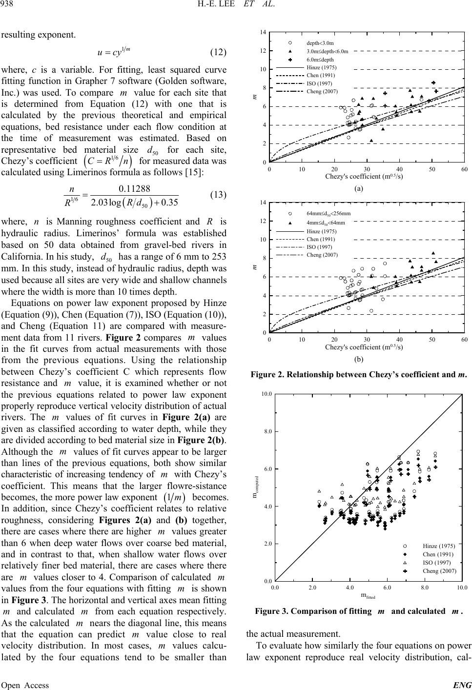 H.-E. LEE ET AL. 938 resulting exponen t. 1m ucy (12) where, c is a variable. For fitting, least squared curve fitting function in Grapher 7 software (Golden software, Inc.) was used. To compare value for each site that is determined from Equation (12) with one that is calculated by the previous theoretical and empirical equations, bed resistance under each flow condition at the time of measurement was estimated. Based on representative bed material size 50 for each site, Chezy’s coefficient m d 16 CRn for measured data was calculated using Limerinos formula as follows [15]: 16 50 0.11288 2.03log 0.35 n Rd R (13) where, is Manning roughness coefficient and is hydraulic radius. Limerinos’ formula was established based on 50 data obtained from gravel-bed rivers in California. In his study, 50 has a range of 6 mm to 253 mm. In this study, instead of hydraulic radius, depth was used because all sites are very wide and shallow channels where the width is more than 10 times depth. nR d Equations on power law exponent proposed by Hinze (Equation (9)), Chen (Equation (7)), ISO (Equation (10)), and Cheng (Equation 11) are compared with measure- ment data from 11 rivers. Figure 2 compares values in the fit curves from actual measurements with those from the previous equations. Using the relationship between Chezy’s coefficient C which represents flow resistance and value, it is examined whether or not the previous equations related to power law exponent properly reproduce vertical velocity distribution of actual rivers. The values of fit curves in Figure 2(a) are given as classified according to water depth, while they are divided according to bed material size in Figure 2(b). Although the values of fit curves appear to be larger than lines of the previous equations, both show similar characteristic of increasing tendency of with Chezy’s coefficient. This means that the larger flowre-sistance becomes, the more power law exponent m m m m m 1 m m 0 1020304050 Chezy'scoefficient ( 60 0.5 /s) 0 2 4 6 8 10 12 14 m depth 3.0m 3.0m depth 6.0m 6.0m depth Hinze (1975) Chen (1991) ISO (1997) Cheng (2007) (a) 0 1020304050 Chezy'scoefficient (m 0.5 /s) 60 0 2 4 6 8 10 12 1 m 64mm d 50 256mm 4mm d 50 64mm Hinze (1975) Chen (1991) ISO (1997) Cheng (2007) (b) Figure 2. Relationship between Chezy’s coefficient and m. 0.0 2.0 4.0 6.0 8.010.0 m itted 0.0 2.0 4.0 6.0 8.0 10.0 m computed Hinze (1975) Chen (1991) ISO (1997) Cheng (2007) m becomes. In addition, since Chezy’s coefficient relates to relative roughness, considering Figures 2(a) and (b) together, there are cases where there are higher values greater than 6 when deep water flows over coarse bed material, and in contrast to that, when shallow water flows over relatively finer bed material, there are cases where there are values closer to 4. Comparison of calculated values from the four equations with fitting is shown in Figure 3. The horizontal an d vertical axes mean fitting and calculated from each equation respectively. As the calculated nears the diagonal line, this means that the equation can predict value close to real velocity distribution. In most cases, values calcu- lated by the four equations tend to be smaller than m m m m m mm Figure 3. Comparison of fitting and calculated . m m the actual measurement. To evaluate how similarly the four equations on power law exponent reproduce real velocity distribution, cal- Open Access ENG 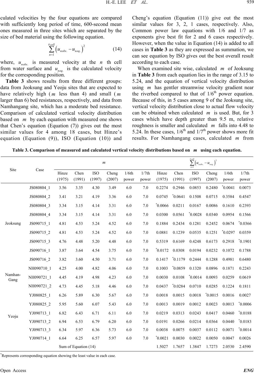 H.-E. LEE ET AL. 939 culated velocities by the four equations are compared with sufficiently long period of time, 600-second mean ones measured in three sites which are separated by the size of bed material using the following equation. #2 .. 1 cell nobs neq n uu (14) where, .nobs is measured velocity at the th cell from water surface and .neq is the calculated velocity for the corresponding position. un u Table 3 shows results from three different groups: data from Jeoksung and Yeoju sites that are expected to have relatively high ( less than 4) and small ( larger than 6) bed resistances, respectively, and data from Namhangang site, which has a moderate bed resistance. Comparison of calculated vertical velocity distribution based on by each equation with measured one shows that Chen’s equation (Equation (7)) gives out the most similar values for 4 among 18 cases, but Hinze’s equation (Equation (9)), ISO (Equation (10)) and m m m Cheng’s equation (Equation (11)) give out the most similar values for 3, 2, 1 cases, respectively. Also, Common power law equations with 1/6 and 1/7 as exponents give best fit for 2 and 6 cases respectively. However, when the value in Equation (14) is added to all cases in Table 3 as they are expressed as summation, we can see equation by ISO gives out the best overall result according to each case. When examined site wise, calculated of Jeoksung in Tabl e 3 from each equation lies in the range of 3.15 to 5.24, and the equation of vertical velocity distribution using has gentler streamwise velocity gradient near the riverbed compared to that of 1/6th power equation. Because of this, in 5 cases among 9 of the Jeoksung site, vertical velocity distribution close to actual flow velocity can be obtained when calculated is used. But, for 3 cases which have depth greater than 9.5 m, relative roughness is smaller and calculated falls into 4.48 to 5.24. In these cases, 1/6th and 1/7th power shows more fit results. For Namhangang cases, calculated m from m m m m Table 3. Comparison of measured and calculated vertical velocity distributions based on using each equation. m m #2 .. 1 cell nobs neq n uu Site Case Hinze (1975) Chen (1991) ISO (1997) Cheng (2007) 1/6th power 1/7th power Hinze (1975) Chen (1991) ISO (1997) Cheng (2007) 1/6th power 1/7th power JS080804_1 3.56 3.35 4.30 3.49 6.0 7.0 0.22740.29460.0853 0.2480 *0.0041 0.0073 JS080804_2 3.41 3.21 4.19 3.36 6.0 7.0 0.0745*0.06410.1508 0.0715 0.35840.4547 JS080804_3 3.34 3.15 4.14 3.31 6.0 7.0 *0.00660.02110.0167 0.0086 0.16100.2393 JS080804_4 3.34 3.15 4.14 3.31 6.0 7.0 0.03000.0561*0.0028 0.0340 0.09540.1566 JS090715_1 4.81 4.53 5.24 4.52 6.0 7.0 0.18840.24340.1281 0.2452 0.0674*0.0366 JS090715_2 4.81 4.53 5.24 4.52 6.0 7.0 0.08810.12390.0535 0.1251 *0.0297 0.0359 JS090715_3 4.76 4.48 5.20 4.48 6.0 7.0 0.53190.61690.4248 0.6173 0.2918*0.1901 JS090716_1 3.87 3.64 4.54 3.75 6.0 7.0 *0.01720.03080.0194 0.0232 0.10720.1788 Jeoksung JS090716_2 3.82 3.60 4.50 3.71 6.0 7.0 0.1417*0.11790.2444 0.1288 0.49810.6480 NH090710_1 4.25 4.00 4.82 4.06 6.0 7.0 0.1003*0.08590.1320 0.0896 0.18710.2243 NH090721_1 4.45 4.19 4.98 4.23 6.0 7.0 0.00300.0108*0.0014 0.0093 0.02590.0619 Namhan- Gang NH090721_2 4.73 4.45 5.18 4.46 6.0 7.0 0.0437*0.02840.0710 0.0285 0.12240.1811 YJ080825_1 6.26 5.89 6.30 5.67 6.0 7.0 0.00180.00150.0018 *0.0015 0.00160.0027 YJ080825_2 5.95 5.60 6.07 5.43 6.0 7.0 0.00130.00190.0012 0.0023 0.0013*0.0006 YJ090713_1 6.82 6.43 6.71 6.11 6.0 7.0 0.02190.03130.0243 0.0417 0.0460*0.0188 YJ090713_2 6.94 6.53 6.79 6.20 6.0 7.0 0.01910.02660.0214 0.0364 0.0440*0.0183 YJ090713_3 6.34 5.97 6.36 5.73 6.0 7.0 0.00380.00750.0037 0.0112 0.0071*0.0014 Yeoju YJ090714_1 6.64 6.25 6.57 5.97 6.0 7.0 *0.00210.00300.0022 0.0050 0.00470.0026 Sum of Equation (14) 1.50271.76571.3847 1.7273 2.05302.4590 *Represents corresponding equation showing the least value in each case. Open Access ENG 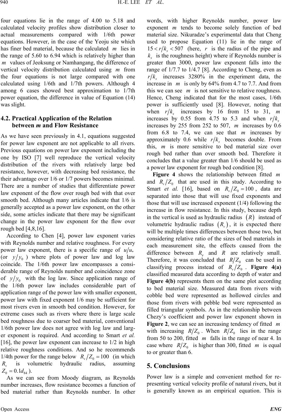 H.-E. LEE ET AL. 940 four equations lie in the range of 4.00 to 5.18 and calculated velocity profiles show distribution closer to actual measurements compared with 1/6th power equations. However, in the case of the Yeoju site which has finer bed material, because the calculated lies in the range of 5.60 to 6.94 which is relatively higher than values of Jeoksung or Namhangang, the difference of vertical velocity distribution calculated using from the four equations is not large compared with one calculated using 1/6th and 1/7th powers. Although 4 among 6 cases showed best approximation to 1/7th power equation, the difference in value of Equation (14) was slight. m m m 4.2. Practical Application of the Relation between m and Flow Resistance As we have seen previously in 4.1, equations suggested for power law exponent are not applicable to all rivers. Previous equations on power law exponent including the one by ISO [7] well reproduce the vertical velocity distribution of the rivers with relatively large bed resistance, however, with decreasing bed resistance, the their advantage over 1/6 or 1/7 powers becomes minimal. There are a number of studies that differentiate power law exponent of the flow over rough bed with that over smooth bed. Although many articles indicate that 1/6 is generally accepted as a power law exponent, on the other side, some articles indicate that there may be significant change in the power law exponent for the flow over rough bed [4,8,16]. According to Chen [4], power law exponent varies with Reynolds number and relative roughness. For every power law exponent, there is a specific range of * uu (or 0 yy ) where plots of power law and log law coincide. The 1/6th power law encompasses a consi- derable range of Reynolds number and coincidence zone of 0 yy with the log law. Since application range of the 1/6th power law includes considerable part of application range of the power law with smaller expon ent, power law with fixed exponent 1/6 may be sufficient for most rivers even in smooth bed condition. However, for extreme cases such as rivers where there is large scale bed roughness due to coarser bed material, conventional 1/6th power law does not agree with log law and larg- er exponent is required. And according to Smart et al. [16], the power law exponent can increase to 1/2 in high relative roughness conditions. And so he recommends 1/4th power for the range below 0100 v RZ (in which is volumetric hydraulic radius, assuming v R 08 0.1 4 d). As we can see from Moody diagram, as Reynolds number increases, flow resistance becomes a function of bed material rather than Reynolds number. In other words, with higher Reynolds number, power law exponent tends to become solely function of bed material size. Nikuradze’s experimental data that Cheng used to propose Equation (11) lie in the range of m 15 507 s rk (here, is the radius of the pipe and r k is the roughness height) where if Reynolds number is greater than 3000, power law exponent falls into the range of 1/7.7 to 1/4.7 [8]. According to Cheng, even as rk increases 3280% in the experiment data, the increase in is only by 64% from 4.7 to 7.7. And from this we can see is not sensitive to relative roughness. Hence, Cheng indicated that for the most cases, 1/6th power is sufficiently used [8]. However, noting that when mm rk increases by 16 from 15 to 31, increases by 0.55 from 4.75 to 5.3 and when m rk increases by 255 from 252 to 507, increases by 0.6 from 6.8 to 7.4, we can see that increases by approximately 0.6 while mm rk becomes double. From this, is more sensitive to bed material size over rough bed rather than over smooth bed. Therefore it concludes that a value greater than 1/6 should be used as a power law exponent for rough bed condition [8]. m Figure 4 shows the relationship between fitted and m 0v RZ that are used in this study. According to Smart et al. [16], based on 0100 v RZ, data are separated into those that will use fixed exponents and those that will use increased ex ponent (1/4) fo llowing the increase in flow resistance. In this study, because depth in the vertical is used as hydraulic radius instead of volumetric hydraulic radius , it is expected there will be multiple times differences between those two, but considering relative ratio of the sizes of bed materials in each measurement site, the effects caused from the difference between v and are relatively small. Therefore, it was concluded that R v R RR 0 RZ can be used in classifying process instead of 0v RZ. Figure 4(a) classified measured data according to depth of water and Figure 4(b) represents them on the same plot according to bed material size. Measured data from rivers with cobble bed were represented as hollowed circles and those from rivers with pebble bed were represented as filled triangular symbols. As in the relationship between Chezy’s coefficient and power law exponent shown in Figure 2, we can see an increasing tendency of fitted with increasing m 0 RZ . When 0 lies in the range from 50 to 200, fitted falls in the range of near 4. In case where RZ m 0 RZ is higher than 300, fitted is equal to or greater than 6. m 5. Conclusions Power law is a simple and convenient method for re- presenting v ertical velo city p rof ile of na tural rivers, but it is generally known as an empirical equation. This is Open Access ENG  H.-E. LEE ET AL. 941 101001000 10000 R/Z 0 0 2 4 6 8 10 12 14 m fitted depth 3.0m 3.0m depth 6.0m 6.0m depth (a) 101001000 10000 R/Z 0 0 2 4 6 8 10 12 14 m fitted 64mm d 50 256mm 4mm d 50 64mm (b) Figure 4. The relationship between 0 Z and fitted based on actual measurement. m because there is a relatively weak theoretical background to power law, especially because it seems that there are insufficient bases to apply specific exponents to rivers with specific flow conditions. Because previous equa- tions used to determine power law exponent are derived from relationship with log law or are based on the data acquired from laboratory experiments, in order to apply these equations to natural river flow, it is necessary to obtain suitable assessment. In this study, vertical velo city profile data measured by ADCPs in natural rivers in South Korea were used to evaluate previous methods for determining power law exponent and to find suitable application areas. The followings are the summary and conclusion of this study. First, fitting of power law exponent for the measured vertical velocity data was conducted, followed with comparison of fitted power law exponents with those calculated by the previous four equations. In case of small bed roughness, because changes due to bed resistance were minimal, widely used powers such as Manning’s 1/6 power or Blasius’ 1/7 power compared to exponents calculated from equations were found to give suitable values. However, in cases of rivers in rough bed condition which have higher flow resistance, the valu e of power law exponent increased with flow resistance. This is because vertical velocity distribution of 1/6th and 1/7th power law shows discrepancy with log law in the range in which the effect of flow resistance is higher (that is, in the flow with relatively smaller 0 y) and also it is because larger values of exponents are more suitable in these ranges. Therefore, four previous equations can be viewed as more suitable for rivers in rough bed condition than those in smooth bed condition. Finally, we proposed the practical guide for determining the power law ex- ponent appropriate for various flow conditions from vertical velocity distributions measured in natural river channels. m 6. Acknowledgements This research was supported by Korea Institute of Construction Technology (Project name: Development of Floodplain Maintenance Technology for Enhancement of Waterfront Values, Project number: 2013-0327). REFERENCES [1] ISO, “Hydrometry-Measuring River Velocity and Dis- charge with Acoustic Doppler Profilers,” International Organization for Standardization, Geneva, Switzerland, ISO/TS 24154, 2005. [2] J. A. Gonzalez-Castro and M. Muste, “Framework for Estimating Uncertainty of ADCP Measurements from a Moving Boat Using Standardized Uncertainty Analysis,” Journal of Hydraulic Engineering, Vol. 133, No. 12, 2007, pp. 1390-1411. http://dx.doi.org/10.1061/(ASCE)0733-9429(2007)133:12 (1390) [3] D. S. Mueller, “extrap: Software to Assist the Selection of Extrapolation Methods for Moving-Boat ADCP Streamflow Measurements,” Computers and Geosciences, Vol. 54, 2013, pp. 211-218. http://dx.doi.org/10.1016/j.cageo.2013.02.001 [4] C.-L. Chen, “Unified Theory on Power Laws for Flow Resistance,” Journal of Hydraulic Engineering, Vol. 117, No. 3, 1991, pp. 371-389. http://dx.doi.org/10.1061/(ASCE)0733-9429(1991)117:3( 371) [5] B. C. Yen, “Open Channel Flow Resistance,” Journal of Hydraulic Engineering, Vol. 128, No. 1, 2002, pp. 20-39. http://dx.doi.org/10.1061/(ASCE)0733-9429(2002)128:1( 20) [6] J. O. Hinze, “Turbulence,” McGraw-Hill Book Co., New York, 1975. [7] ISO, “Measurement of Liquid Flow in Open Channels: Velocity-Area Methods,” International Organization for Standardization, Geneva, Switzerland, ISO 748, 1997. [8] N.-S. Cheng, “Power-Law Index for Velocity Profiles in Open Channel flows,” Advances in Water Resources, Vol. Open Access ENG  H.-E. LEE ET AL. Open Access ENG 942 30, No. 8, 2007, pp. 1775-1784. http://dx.doi.org/10.1016/j.advwatres.2007.02.001 [9] J. A. González-Castro, C. S. Melching and K. A. Oberg, “Analysis of Open-Channel Velocity Measurements Col- lected with an Acoustic Doppler Current Profiler,” 1st In- ternational Conference on New/Emerging Concepts for Rivers, RIVERTECH 96, IWRA, Chicago, 22-26 Sep- tember 1996, pp. 838-845. [10] M. Muste, K. Yu and M. Spasojevic, “Practical Aspects of ADCP Data Use for Quantification of Mean River Flow Characteristics; Part I: Moving-Vessel Measure- ments,” Flow Measurement and Instrumentation, Vol. 15, 2004, pp. 1-16. [11] M. Muste, K. Yu and M. Spasojevic, “Practical Aspects of ADCP Data Use for Quantification of Mean River Flow Characteristics; Part II: Fixed-Vessel Measure- ments,” Flow Measurement and Instrumentation, Vol. 15, 2004, pp. 17-28. [12] D. Kim, M. Muste, J. A. González-Castro and M. Ansar, “Graphical User Interface for ADCP Uncertainty Analy- sis,” Proceedings of the ASCE World Water and Envi- ronmental Resources Congress, Anchorage, 15-19 May 2005, pp. 1-12. [13] J. Le Coz, G. Pierrefeu and A. Paquier, “Evaluation of River Discharges Monitored by a Fixed Side-Looking Doppler Profiler,” Water Resources Research, Vol. 44, 2008, Article ID: W00D09. http://dx.doi.org/10.1029/2008WR006967 [14] P. M. Pelletier, “Uncertainties in the Single Determina- tion of River Discharge: A Literature Review,” Canadian Journal of Civil Engineering, Vol. 15, No. 5, 1988, pp. 834-850. http://dx.doi.org/10.1139/l88-109 [15] J. T. Limerinos, “Determination of the Manning Coeffi- cient from Measured Bed Roughness in Natural Chan- nels,” U.S. Geological Survey Water-Supply Paper 1898- B, 1970. [16] G. M. Smart, M. J. Duncan and J. M. Walsh, “Relatively Rough Flow Resistance Equations,” Journal of Hydraulic Engineering, Vol. 128, No. 6, 2002, pp. 568-578. http://dx.doi.org/10.1061/(ASCE)0733-9429(2002)128:6( 568)
|