Advances in Applied Sociology
2013. Vol.3, No.7, 289-300
Published Online November 2013 in SciRes (http://www.scirp.org/journal/aasoci) http://dx.doi.org/10.4236/aasoci.2013.37037
Open Access 289
Understanding the Linkages of Household Environmental
Deprivation, Asset Index and Child Survival in India
Bidyadhar Dehury
International Institute for Population Sciences, Mumbai, India
Email: bidyadehury@gmail.com
Received October 2nd, 2013; revised November 2nd, 2013; accepted November 9th, 2013
Copyright © 2013 Bidyadhar Dehury. This is an open access article distributed under the Creative Commons
Attribution License, which permits unrestricted use, distribution, and reproduction in any medium, provided the
original work is properly cited.
Often the household environmental factors are combined with the household assets in explaining the eco-
nomic differentials in population and health parameters of developing countries. Though the utility of
wealth index (that combines household environment with assets) in explaining health and health care
utilization is established, its utility as a proxy of economic measures is contested. In this paper we at-
tempted to differentiate the role of household environmental factors and the household assets in explain-
ing the infant mortality (IMR) and the under-five mortality (U5MR) in India. We hypothesize that there
are no significant differences in IMR and U5MR among those households residing in poor household en-
vironmental condition and those who are poor in asset in India. We have used the data from the National
Family Health Survey (NFHS-3), 2005-06, India, a population based large scale representative survey.
Bi-variate analyses, principal component analysis, life-table technique and hazard model are used in the
analyses. Two composite indices namely, an asset index based on consumer durables of the households
and household environmental deprivation index based on the household environmental factors are con-
structed. The indices are categorized as poor and non-poor based on the 50% of the median composite
score. Result shows that the correlation coefficient of asset index and household environmental depriva-
tion index is weak. Further, there are no significant differences of IMR and U5MR among households
living in poor household environment and those are poor in asset cutting across the states. Results of
cox-proportional hazard model indicate that the household environmental factors have significant impact
on child survival. It calls for improving the household environmental conditions of the household in pro-
moting child survival in India.
Keywords: Household Environmental Deprivation; Asset Index; Child Survival; IMR;
U5MR; Urban India
Introduction
To improve child survival, measurement by reduction of in-
fant and under-five mortality are two monitoring indicators of
the Millennium Development Goals (MDGs). Empirical evi-
dences across the globe suggest that the progresses in these
indicators are slow and uneven across and within the countries
(Lawn et al., 2006). Though the millennium declaration aimed
to reduce the infant and under-five mortality by two-thirds by
2015 from the base year (1990), many developing countries
including India are lagging behind. According to UNICEF
(2009) though the progress in under-five mortality (U5MR) has
been made in many countries, the global rate of progress is still
insufficient to achieve the MDGs. Africa and Asia combined
account for 93 per cent of all under-five deaths that occur each
year in the developing world and India accounts about one-fifth
of global under-five mortality, which is more than any other
country (Black et al., 2010). During 1992-93 and 2005-06, the
infant mortality rate (IMR) in India had declined from 79 to 57
per 1000 live births while the under-five mortality rate had de-
clined from 109 to 74 per 1000 live births (IIPS and Macro In-
ternational, 2007). However, the actual rate of progress in re-
duction of infant and under-five mortality is lower than the
required rate of progress for the country (Ram et al., 2008). The
MDG target to reduce the IMR by 27 and U5MR by 41 seems
unattainable for the country by 2015 and the global effort in
achieving the MDGs is largely contingent on India’s success
(You et al., 2010).
The child survival, particularly during infancy is broadly af-
fected by a set of endogenous and exogenous factors. Endoge-
nous factors are mainly biological and arise from genetic causes
such as congenital disorders, premature births, birth injuries etc.
On the other hand, the exogenous factors are mainly environ-
mental or external factors that cause infections and accidents. It
is evident that in developing countries most of the deaths among
under-five years are associated with the infectious diseases
mainly caused by the poor household environmental conditions
(Sastry, 1996; Muhuri, 1996; Ayad et al., 1997; Hoque et al.,
1999; Folasade, 2000; Anderson et al., 2002; Mutunga, 2007;
Kembo & Ginneken, 2009; Fink et al., 2011; Cheng et al., 2012).
An estimated 1.87 million children aged below five years in de-
veloping countries died in 2004 due to diarrhea (Boschi-Pinto,
2008). Pruss et al. (2002) estimated that 4% of all deaths (in-
cluding children) and 5.7% of total disability-adjusted life years
can be attributed to water, sanitation, and hygiene. Cheng et al.
B. DEHURY
(2012) found that increase in access to water and sanitation
leads to significant decrease in IMR and U5MR. The world
health organization (WHO) estimated about 3.5 million deaths
and one tenth of global disease burden could be prevented
worldwide annually by improving water supply, sanitation, hy-
giene and management of water resources (Pruss-Ustun et al.,
2008). The use of biomass as cooking fuel results in air dense
with particulates and gases which affect the lungs and lives. In
developing countries, the indoor air pollution leads to a higher
chance of respiratory diseases and causes about 2 million deaths
annually to children under-five years of age (WHO, 2007). It
was estimated that the indoor air pollution caused by traditional
cooking fuel is responsible for 3.7% of the loss of disability
adjusted life years in developing world (WHO, 2007). However,
the deaths due to environmental factors are viewed as relatively
preventable and treatable (Pruss-Ustun et al., 2008).
Often the household environmental factors are combined
with the household assets in explaining the economic differen-
tials in population and health parameters of developing coun-
tries. Though the utility of asset index (that combines house-
hold environment with assets) in explaining health and health
care utilization is established, its utility as a proxy of economic
measures is contested. Theoretically, the households which are
economically stronger are likely to have better household envi-
ronmental condition. But this may not be always true. We be-
lieve that the economic proxies (consumer durables) of the
household are necessary but not sufficient condition in promot-
ing child survival. Also, little is known on the association of
household environmental conditions and economic conditions
of the households at disaggregated level. Moreover, the econo-
mic conditions measured by economic proxies (also refereed as
household asset) are basic necessities of life and often inherited
from parents or relatives.
In this paper we attempted to differentiate the role of house-
hold environmental factors and the household assets in ex-
plaining the infant mortality (IMR) and the under-five mortality
(U5MR) in India. We hypothesize that there are no significant
differences in child survival among the households residing in
poor household environmental condition and they are proof in
asset. This is primarily because 1) a sizeable proportion of po-
pulation residing in poor household environmental condition
such as slums have many of the household assets 2) the vari-
ables used in the asset index do not adequately measure the
household wealth 3) the child health is very sensitive to the
environmental condition of the households, such as water con-
tamination, cooking fuel, sanitary facilities etc. The present
study aims to understand the role of household environmental
deprivations on child survival in India.
The paper has three specific objectives. The first objective is
to examine the association of household environmental depri-
vations and household asset, the second objective is to estimate
the infant and under five mortality rate by household environ-
mental conditions and household asset index, and the third ob-
jective is to examine the factors associated with child survival
(IMR and under five mortality).
Data and Methods
Data
The unit data from National Family Health Survey (NFHS-3),
conducted in 2005-06 is used in the analyses. The NFHS-3 is a
nationally representative population based survey that success-
fully interviewed 109,414 households and 124,385 women. Two
sets of questionnaires, namely, the household questionnaire and
women questionnaire were used in the survey. The household
questionnaire collected information of household environmen-
tal conditions such as drinking water, dwelling conditions (ma-
terial used for wall, floor and roof), electrification, cooking fuel,
cooking arrangement, window in the house and ownership of
consumer durables. This information is used to construct the
household environmental deprivation index and an asset index
for the household. The women questionnaire collected informa-
tion on fertility, contraception, nutrition etc from the selected
women. From the birth histories of women, kids file and birth
history file are prepared. We have used the births of last five
years to estimate the IMR and births of last 10 years to estimate
the under-five mortality.
Methods
The Principal Component Analysis (PCA) is used to con-
struct the household environmental deprivation index and an
asset index of the households, separately for rural and urban
areas. This is because the health estimates differ significantly
when separate wealth index for rural and urban areas are used
against single wealth index (Mohanty, 2009). PCA assigns
weight to each of the variables in constructing composite index.
A positive weight indicates the better economic status and a
negative weight indicates relatively lower economic status. In
construction of composite indices, the variables are re-coded in
a binary form (0 and 1). In construction of asset index for rural
areas, ownership of house is not included and for the urban
asset index, the ownership of land is not included. The compos-
ite indices are categorized into two, namely, the poor and non-
poor. The cut-off point of poor is based on 50% of the median
composite score and all other were classified as non-poor.
Bivariate analyses and correlation coefficient are used to un-
derstand the association of asset index and the household envi-
ronmental deprivation index. The alpha test is used to check the
reliability of the estimates and Z test is used to test the signifi-
cance difference in estimates. The life table technique is used to
derive the estimates of IMR and U5MR among poor and non-
poor, for both household environmental deprivation index and
asset index. The cox-proportional hazard model is used to un-
derstand the significant predictor of child survival. The com-
bined estimates are derived from rural and urban estimates and
the analyses are carried out for India and major states. The in-
fant mortality rate is estimated from the kid’s file that depicts
the birth history of the women in five years preceding the sur-
vey. The under-five mortality rate is estimated from ten years
birth history of women preceding the survey from the birth file.
Results
Household Environmental Deprivation Index
and Asset Index
Table 1 describes the mean, standard deviation and factor
score of household environmental deprivations, separately for
rural and urban India. The distribution of variables on house-
hold environmental conditions is skewed, both in rural and ur-
ban areas. For example, the distribution of households on
drinking water showed that 72% of household in urban India
used piped water followed by tube well, dug well and other
Open Access.
290
B. DEHURY
Open Access 291
Table 1.
Mean, standard deviation and factor score of variables used in computation of household environmental deprivation index in urban India, 2005-06.
Urban Rural
Household Variable s Mean Standard DeviationFactor Scor e Mean Standard Deviation Factor Score
Sources of Drinking Water
Piped water .719 .449 .145 .281 .450 .196
Tube well .213 .409 .133 .532 .499 .176
Dug well .048 .213 .041 .155 .361 .011
Other sources .020 .140 .011 .033 .178 .022
Electricity .931 .254 .242 .558 .497 .280
Type of Toilet
Flush toilet .787 .410 .336 .200 .400 .337
Pit toilet .040 .196 .077 .059 .236 .029
No toilet/open field .172 .378 .325 .740 .439 .323
Type of Cooking Fuel
Electricity/biogas .601 .490 .340 .088 .283 .316
Biomass .261 .439 .328 .891 .311 .328
Kerosene/charcoal .138 .345 .066 .021 .142 .088
Has Window .847 .360 .269 .586 .493 .279
Material Used in the House
Finished material used for wall .889 .314 .268 .534 .499 .268
Finished material used for floor .807 .395 .275 .305 .460 .323
Finished material used for roof .924 .265 .231 .714 .452 .216
Persons Per Sleeping Room
<2 persons .377 .485 .102 .325 .468 .110
2 - 5 persons .534 .499 .038 .543 .498 .034
>5 persons .089 .285 .106 .132 .338 .102
Cooking Arrangement
No separate kitchen .272 .445 .183 .339 .474 .183
Separate kitchen .590 .492 .288 .341 .474 .235
Separate building .043 .204 .026 .099 .298 .012
Outdoor .093 .291 .188 .220 .414 .069
ALPHA .784 .762
sources. Similarly, 79% of urban households used flush toilet
and 17% didn’t had any toilet. About three-fifths of urban
households used electricity and biogas as cooking fuel. The
standard deviation varies substantially indicating the variability
within the urban areas. The factor score of the variables are in
expected ways both in rural and urban areas. For example, the
factor score of electricity/biogas is .34 and that of biomass is
.33 in urban areas. The alpha value of household environmen-
tal deprivation index is .784 in urban and .762 in rural India
indicating that the estimates are reliable. Figures 1 and 2 shows
the distributions of household environmental deprivation index
for urban and rural India respectively. While the distribution of
household environmental deprivation score is less skewed in
rural areas, it is more skewed in urban areas.
Table 2 describes the mean, standard deviation and factor
score of asset index separately for urban and rural India. It may
be mentioned that the variables used in the asset index are eco-
nomic proxies and not the direct measure of economic status of
B. DEHURY
Figure 1.
Distribution of household environmental deprivation index in ur-
ban India, 2005-06.
Figure 2.
Distribution of household environmental deprivation index in
rural India, 2005-06.
the households. The distribution of households on ownership of
consumer durables in urban India showed that it was maximum
for watch (91%) followed by cot (86%), fan (85%) and chair
(76%) and minimum for agricultural accessories, probably be-
cause large proportion of households in urban areas worked in
non-agricultural activities. The standard deviation varies from .5
for bicycle and color television to a minimum for thresher (.065)
and tractor (.068). Similarly in rural India about 81% of house-
holds own a cot followed by own a watch (71%), own a bicycle
(51.5%) and own mattress (48.6%). The standard deviation of
variables is maximum in mattress and bicycle (.5) followed by
marginal land, no land holdings and chair (.49). The factor
scores of the variables are positive except no land and marginal
land. These groups are poorest as compared to medium and
large land holdings. The distribution of asset index for urban
and rural India is given in Figures 3 and 4 respectively. It is ne-
gatively skewed in rural areas and normal in urban areas. The
alpha value of asset index is .85 in urban and .82 in rural India.
Table 3 provides the cross classification of households in
asset index and household environmental deprivation index by
place of residence in India. Our interest is to examine the extent
of association of household environmental deprivation index
and asset index. We have hypothesized that people possessing
asset measured by economic proxies not necessarily reside in
good household environmental condition. Moreover, studies
Figure 3.
Distribution of asset index in urban India, 2005-06.
Figure 4.
Distribution of asset index in rural India, 2005-06.
indicate that the agreement of consumption expenditure and
economic proxies in India are not strong in Indian context
(Srivastava & Mohanty, 2010). Because many of the variables
used in asset index are necessity of life and often inherited. The
results indicate that in India about 79.2% households who are
asset poor, resides in poor household environmental condition
but 27.7% of non-poor also resides in poor household environ-
mental conditions. This is higher in rural areas than urban areas.
The correlation coefficient of asset index and household envi-
ronmental deprivation index is .51; .61 for urban and .48 for
rural India indicating weak association of asset index and house-
hold environmental deprivation index.
Table 4 provides the correlation coefficient of household de-
privation index and asset index by place of residence in the
states of India. The correlation coefficient of asset index and
household environmental deprivation index varies from .60 in
the state of Odisha to .33 in the state of Jammu & Kashmiri. In
urban India the correlation coefficient varies from .71 in Chhat-
tisgarh to .34 in Sikkim. Likewise, in rural India the maximum
correlation is found in Odisha (.57) and minimum in Delhi (.22).
It shows that the association of two indices is generally low and
lower in the rural areas than the urban areas, in most of the
states.
Estimate of Infant and Under- Five M ort al ity Rate by
Household Environmental Deprivation Index
and Asset Index
Table 5 provides the estimates of IMR and U5MR for each
Open Access.
292
B. DEHURY
Open Access 293
Table 2.
Mean, Standard Deviation (SD) and factor score of variables used in computation of asset index in India, 2005-06.
Urban Rural
Wealth Variables Mean Standard De viationFactor Scor eMeanStandard De viation Factor Score
Own a house .783 .413 .074 - - -
Bank/post office account .574 .495 .250 .327 .469 .226
Mattress .753 .432 .248 .486 .500 .207
Pressure cooker .698 .459 .276 .220 .414 .289
Chair .760 .427 .255 .438 .496 .269
Cot .863 .344 .183 .812 .391 .132
Table .649 .477 .284 .329 .470 .285
Fan .847 .360 .204 .386 .487 .269
Radio .389 .488 .156 .269 .444 .171
B & W Television .256 .436 .060 .186 .390 .135
Color Television .514 .500 .294 .125 .331 .258
Sewing .308 .462 .200 .126 .332 .221
Mobile .362 .481 .265 .073 .261 .231
Telephone .266 .442 .270 .080 .271 .246
Computer .081 .272 .177 .006 .076 .091
Refrigerator .334 .472 .300 .066 .248 .232
Watch .910 .286 .160 .713 .453 .200
Bicycle .501 .500 .084 .515 .500 .112
Scooter .303 .460 .263 .107 .309 .257
Cart .010 .099 .014 .074 .262 .086
Car .061 .239 .169 .010 .099 .124
Pump .110 .313 .152 .099 .298 .169
Thresher .004 .065 .029 .022 .147 .099
Tractor .005 .068 .034 .023 .150 .137
No land - - - .416 .493 .091
Marginal land holdings (0 - 2.5 acres) - - - .392 .488 .020
Small land holdings (2.5 - 5 acres) - - - .082 .274 .130
Medium and large land holdings (>5 acres) - - .110 .313 .060
Irrigated land .380 .485 .115
ALPHA .847 .820
Note: Not used in analysis.
of the variables which are used in construction of household en-
vironmental deprivation index and the asset index. The esti-
mates of child survival by source of drinking water showed that
the estimated IMR among households access to pipe water is 40
compared to 64 for tube well and 55 for dug well. Similar dif-
ferences are observed for U5MR and by place of residence. The
IMR and U5MR are estimated higher among those households
does not have electricity in the household and it is true in rural
and urban areas. The mortality rates are much lower among
those households access to flush toilet followed by pit toilet
households and higher among those households does not have
toilet facility or use open field for defecation. In case of cook-
B. DEHURY
Table 3.
Cross classification of household environmental deprivation index and
asset index by type of place of residence in India, 2005-06.
Asset Index
Household environmental
deprivation index Poor Non poor
Urban
Poor (%) 73.6 13.4
Non-poor (%) 26.4 86.6
N 25,475 23,785
Rural
Poor (%) 81.8 34.7
Non-poor (%) 18.2 65.3
N 30,306 27,463
Combined
Poor (%) 79.2 27.7
Non-poor (%) 2.8 72.3
N 55,888 51,141
ing fuel, the estimated IMR among households using biomass
and kerosene/charcoal is almost double of those households us-
ing biogas. This becomes three times higher in rural areas and
in urban areas it is little less than two times. Similar differ-
entials are observed for U5MR. In case of cooking arrangement,
the estimated IMR among households cooking food within the
household is 49 compared to 53 among those households cook
food in separate house and 64 among those households cook
food outside house. Having window in the households also
show significant differential in IMR and U5MR estimates with
higher among those households do not have window in house.
After examining the individual component, we attempted to
understand the differentials in the estimates of IMR and U5MR
rate separately for urban and rural India by household environ-
mental deprivation index and asset index. From the graphs
(Figures 5 and 6) it is clearly seen that there are no significant
differences in the proportion of child surviving under age five
for both household environmental deprivation index and asset
index. But there are significant differences in child survival be-
tween poor and non-poor households either by household envi-
ronmental poor or asset poor (z test). The proportion of child
survival has decreased rapidly from the birth to age five in case
of either in poor household environmental condition or asset poor
than the non-poor households.
Table 6 describes the differentials in estimated IMR and
U5MR among households reside in poor household environ-
mental condition and asset poor by place of residence. For ex-
ample, the estimated IMR among asset poor and households re-
siding in poor household environmental condition is 62 per
1000 live birth each. Similarly, the U5MR among asset poor is
87 compared to 89 among those residing in poor household en-
vironmental condition. The pattern is similar for rural and urban
areas. However, the poor and non-poor differentials are large
by both household environmental deprivation index and asset
index. For example, the estimated IMR among households
Table 4.
State level correlation of household environmental deprivation index
and asset index by place of residence in India, 2005-06.
Correlation Coefficient
States Urban Rural Combined
Andhra Pradesh .58 .41 .46
Arunachal Pradesh .60 .52 .54
Assam .66 .48 .51
Bihar .63 .48 .50
Chhattisgarh .71 .40 .49
Delhi .63 .22 .62
Goa .58 .48 .55
Gujarat .54 .45 .47
Haryana .55 .37 .43
Himachal Pradesh .46 .35 .36
Jammu & Kashmiri.48 .26 .33
Jharkhand .66 .47 .58
Karnataka .54 .39 .45
Kerala .48 .38 .47
Madhya Pradesh .67 .47 .54
Maharashtra .58 .46 .51
Manipur .51 .45 .52
Meghalaya .42 .51 .47
Mizoram .42 .52 .49
Nagaland .41 .44 .47
Odisha .69 .57 .60
Punjab .65 .38 .52
Rajasthan .63 .46 .52
Sikkim .34 .49 .44
Tamil Nadu .58 .37 .48
Tripura .62 .53 .58
Uttar Pradesh .64 .43 .47
Uttaranchal .65 .45 .49
West Bengal .66 .51 .56
India .61 .48 .52
residing in poor household environmental condition is 62 per
1000 live births compared to 38 among non-poor. The differ-
ences are large in rural areas compared to urban areas. This dif-
ference indicates that the household environmental condition
have significant influence on IMR and U5MR. From the z test
it is found that the calculated values of z test are smaller than
the tabulated value in 95% confidence interval by place of re-
sidence and states in India. We infer that there is not much
Open Access.
294
B. DEHURY
Open Access 295
Table 5.
Estimated IMR and U5MR of household environmental conditions by place of residence in India, 2005-06.
Urban Rural Total
Household variabl e s IMR U5MR IMR U5MR IMR U5MR
Sources of drinking water
Piped water 37 53 46 64 40 57
Tube well 58 69 66 92 64 86
Dug well 43 50 57 83 55 77
Other sources 39 64 49 66 46 66
Electricity
No 61 82 70 102 69 99
Yes 40 54 49 65 45 59
Type of toilet
Flush toilet 39 49 35 47 38 49
Pit toilet 53 79 50 72 51 74
No toilet/open field 54 82 66 92 65 91
Type of cooking fuel
Electricity/biogas 33 40 25 34 32 39
Biomass 55 80 60 86 59 85
Kerosene/charcoal 52 70 72 55 55 68
Window in house
No 58 77 70 104 67 97
Yes 38 51 49 64 44 58
Material used in wall
Finished material 39 52 52 71 45 61
Rudimentary 55 75 62 89 61 86
Material used in floor
Finished material 39 53 43 49 41 52
Rudimentary 51 66 63 92 61 87
Material used in the roof
Finished material 40 53 53 74 48 64
Rudimentary 59 97 68 97 66 97
Cooking arrangement
Inside house (no separate kitchen) 53 70 67 90 62 87
Inside house (separate kitchen) 33 42 47 61 40 51
Separate building 42 40 56 75 53 68
Outdoor 65 94 63 89 64 90
difference in proportion dead among households with poor
household environmental condition and asset poor households
but significant and large differences in child survival among
poor and non-poor households.
B. DEHURY
Figure 5.
Child Survival by Asset Index in India, 2005-06.
Figure 6.
Child Survival by Household Deprivation Index in Urban
India, 2005-06.
Table 6.
Estimated IMR and U5MR by household environmental deprivation
index and asset index by place of residence in India, 2005-06.
Household environmental
deprivation index Asset index
IMR and
U5MR
Poor Non-poor Poor Non-poor
IMR
Rural 69 42 68 48
Urban 50 33 53 29
India 62 38 62 42
U5MR
Rural 100 53 98 58
Urban 72 40 72 34
India 89 46 87 50
Table 7 provides the differential in estimated IMR and
U5MR by asset index and household environmental deprivation
index for states of India. In most of the states, the general pat-
tern holds true, that is, the estimated IMR and U5MR among
the poor are substantially higher than the non-poor, both by
household environmental deprivation index and asset index.
Among the states, the estimated IMR among those living in
poor household environmental condition is maximum in the
state of Uttar Pradesh (82) followed by Chhattisgarh, Rajasthan,
Madhya Pradesh, Arunachal Pradesh and Jharkhand where IMR
is more than 70 per thousand live birth. On the other hand, the
IMR among poor household environmental condition house-
holds is minimum in the state of Goa (8) followed by Kerala
and Tamil Nadu with IMR of 34 each, 37 in Manipur and 38 in
Andhra Pradesh. On the other hand, among asset poor house-
holds the IMR is higher in the state of Punjab where the IMR is
87 per thousand live birth and minimum in the state of Goa
with IMR of 22 per thousand live birth. On comparing the es-
timated IMR among asset poor and poor household environ-
mental condition we found that the states such as Andhra Pra-
desh, Haryana, Jammu and Kashmiri, Kerala, Mizoram, Odisha,
Rajasthan, Sikkim, Uttar Pradesh and Chhattisgarh have higher
IMR among those reside in poor household environmental con-
dition than that of asset poor. Among these states Jammu and
Kashmiri has the maximum difference with 21 points difference
of IMR between poor household environmental households and
asset poor households. Similarly the states like Bihar, Jhark-
hand and Tamil Nadu have no difference in IMR between asset
poor households and poor household environmental condition
households. From the table it is also found that most of the
states have higher U5MR rates among the households living in
poor household environmental condition compared to those are
asset poor. There are two states found; Madhya Pradesh and
Uttar Pradesh where there is no difference in U5MR between
those households living in poor household environmental con-
dition compared to asset poor households.
Factors Affecting Child Survival
Table 8 presents the results of Cox Proportional Hazard mo-
del to understand the significant predictor of child survival se-
parately for rural and urban India. Time is the dependent vari-
able and death is the failure variable (0 for surviving and 1 for
dead). The independent variables are a set of demographic and
social variables, namely, age at birth, education of the mother,
preceding birth interval, place of delivery, type of birth (single
or multiple), duration of breastfeeding, working status of mo-
ther, body mass index of mother, sex of the child, caste of mo-
ther and place of residence. Additionally, the household envi-
ronmental deprivation index and the asset index are included in
the hazard model. Results indicate that mother’s education, sex
of the child, preceding birth interval, place of delivery, type of
birth, duration of breastfeeding are significant predictors of
child survival in India. Along with these confounders house-
hold environmental deprivation is also found a strong predictor
of child survival in India and also in both rural and urban India.
The relative hazard ratio is .687 [.566 - .835] for the non-poor
households compared to those who are poor in household envi-
ronmental condition. The hazard ratio is higher in rural areas
compared to the urban areas. On the other hand, the relative
hazard ratio among the asset non-poor is .854 [.717-1.017]
compared to those who are asset poor households. The relative
hazard ratio is not significant in both rural and urban areas. In
the level of education of mothers it is found that the relative
hazard ratio is less for the educated mothers than the unedu-
cated mothers. The relative risk is .46 for mothers with secon-
dary and higher education compared to mothers with no educa-
tion. The hazard ratio is significantly higher for female child
compared to male child. The preceding birth interval also has
greater influence on child survival. The relative risk of hazard
Open Access.
296
B. DEHURY
Open Access 297
Table 7.
State level estimated IMR and U5MR by household environmental deprivation index and asset index in India, 2005-06.
IMR U5MR
Household environmental
deprivation index Asset index Household environmental
deprivation index Asset index
STATES
Poor Non-poor PoorNon-poorDa Poor Non-poor Poor Non-poor Db
Andhra Pradesh 38 44 35 47 03 66 50 52 64 14
Arunachal Pradesh 73 45 84 40 10141 78 157 69 17
Assam 70 61 81 53 1190 55 102 47 13
Bihar 65 47 65 58 00 89 60 93 59 04
Chhattisgarh 80 40 73 72 07 106 59 102 85 04
Delhi 57 38 60 32 0374 33 69 34 05
Goa 8 18 22 13 1466 25 86 16 20
Gujarat 61 42 66 39 0584 48 80 52 03
Haryana 67 31 49 41 17 79 42 64 54 15
Himachal Pradesh 42 29 50 29 0860 38 54 41 05
Jammu and Kashmir 64 38 43 49 21 77 42 53 55 24
Jharkhand 71 51 71 60 00 101 67 102 72 01
Karnataka 47 43 54 36 0871 54 82 35 11
Kerala 34 11 33 12 01 14 13 32 8 18
Madhya Pradesh 73 44 80 40 07112 50 112 49 00
Maharashtra 40 36 46 29 0661 43 68 33 06
Manipur 37 26 49 19 1161 49 83 37 21
Meghalaya 42 52 45 49 0385 36 71 51 14
Mizoram 42 27 36 32 06 55 31 40 44 15
Nagaland 51 31 54 27 0369 50 66 55 03
Odisha 61 65 60 68 01 90 64 96 58 06
Punjab 59 38 87 31 2873 49 77 51 03
Rajasthan 77 51 76 58 01 104 66 107 66 03
Sikkim 49 31 39 32 10 57 35 31 44 25
Tamil Nadu 34 30 34 27 00 57 38 59 22 02
Tripura 53 51 56 47 0278 58 91 43 13
Uttar Pradesh 82 47 81 65 01 120 58 120 86 00
Uttarakhand 58 31 61 36 0283 61 109 52 25
West Bengal 50 45 53 39 0460 46 62 39 01
India 62 38 62 42 00 89 46 87 50 02
Note: aDifferences in IMR of household environmental deprivation index (poor) and asset index (poor); bDifferences in U5MR of household environmental deprivation
index (poor) and asset index (poor).
decreases with increase in the preceding birth interval. The
relative risk is significantly higher (3.1 times) for multiple birth
compared to the single birth. The duration of breastfeeding is
also a significant predictor of child survival. In urban India,
mother’s education for secondary and higher, preceding birth
interval, type of birth, duration of breastfeeding, working status
B. DEHURY
Table 8.
Hazard ratio and 95% confidence interval of mortality under ages five in India, 2005-06.
Hazard ratio 95% Confidence interval
Covariates
Urban Rural Total Urban Rural Total
Place of residence
Urban®
Rural - - 1.145 .963 - 1.361
Household e nvironmental depri va tion index
Poor®
Non-poor .687* .694*** .687*** .464 - 1.018 .554- .870 .566 - .835
Asset index
Poor®
Non-poor .830 .863 .854* .557 - 1.237 .709 - 1.050 .717 - 1.017
Age at birth
<19®
20 - 29 1.316 .796* .887 .743 - 2.330 .607 - 1.044 .695 - 1.132
30+ 1.559 1.052 1.141 .833- 2.916 .777 - 1.425 .870 - 1.497
Education of m ot her
No education® .973 .718** .797** .685 - 1.381 .556 - .928 .649 - .978
Primary .370*** .538*** .466*** .255 - .536 .411 - .703 .375 - .580
Secondary/higher
Sex of the child
Male®
Female 1.198 1.308*** 1.270*** .921 - 1.559 1.109 - 1.543 1.104 - 1.460
Preceding birth interval
<2 years® .684** .657*** .654*** .497 - .941 .543 - .795 .555 - .770
2 - 3 years .505*** .470*** .474*** .360 - .708 .378 - .584 .395 - .569
3+ years
Place of delivery
Home®
Hospital .733** .623*** .657*** .541 - .992 .479 - .811 .540 - .800
Caste
SCs® 1.246 1.011 1.020 .811 - 1.915 .795 - 1.286 .828 - 1.257
STs .840 .845 .837* .592 - 1.191 .673 - 1.060 .692 - 1.012
OBC .704** 1.022 .895 .479 - 1.035 .792 - 1.319 .723 - 1.106
Others
Type of birth
Single birth®
Multiple birth 2.979*** 3.065*** 3.110*** 1.425 - 6.227 2.088 - 4.498 2.222 - 4.377
Working status of mother
Open Access.
298
B. DEHURY
Continued
No®
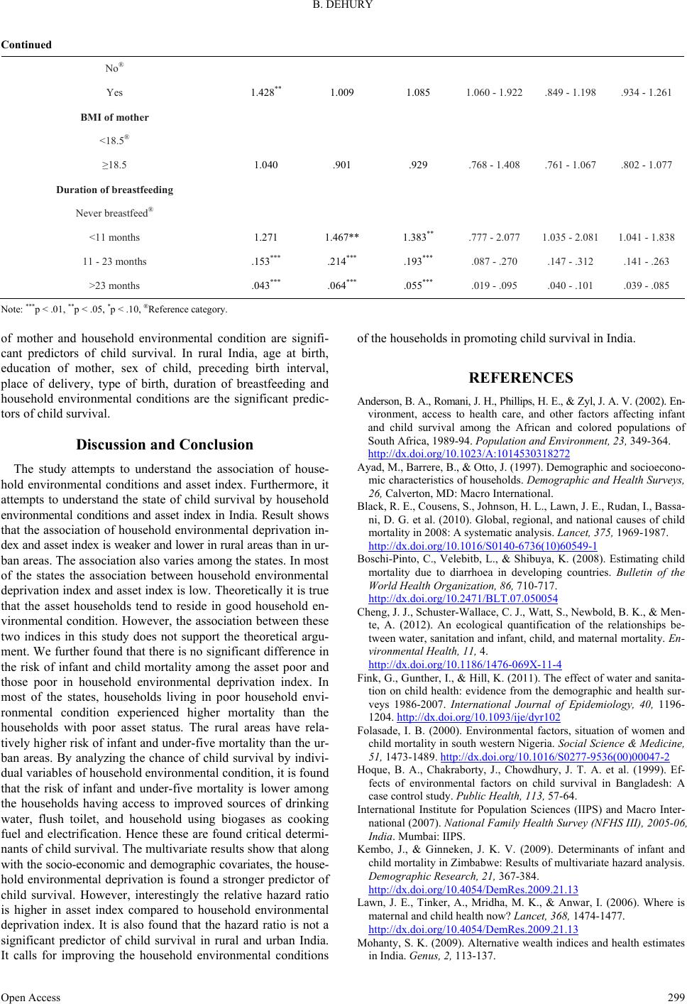
Yes 1.428** 1.009 1.085 1.060 - 1.922 .849 - 1.198 .934 - 1.261
BMI of mother
<18.5®
18.5 1.040 .901 .929 .768 - 1.408 .761 - 1.067 .802 - 1.077
Duration of breastfeeding
Never breastfeed®
<11 months 1.271 1.467** 1.383** .777 - 2.077 1.035 - 2.081 1.041 - 1.838
11 - 23 months .153*** .214*** .193*** .087 - .270 .147 - .312 .141 - .263
>23 months .043*** .064*** .055*** .019 - .095 .040 - .101 .039 - .085
Note: ***p < .01, **p < .05, *p < .10, ®Reference category.
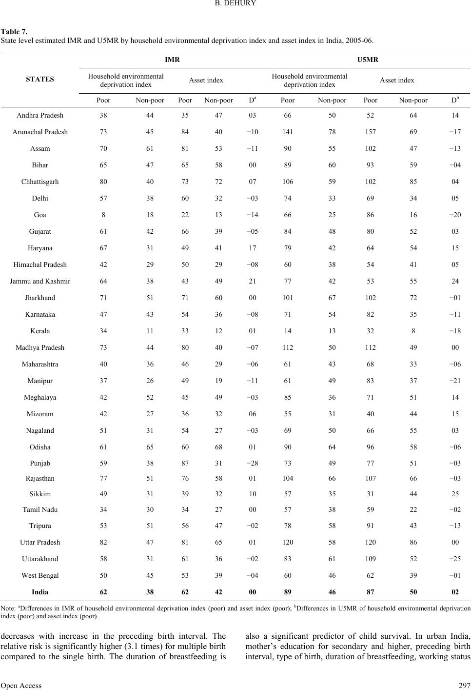
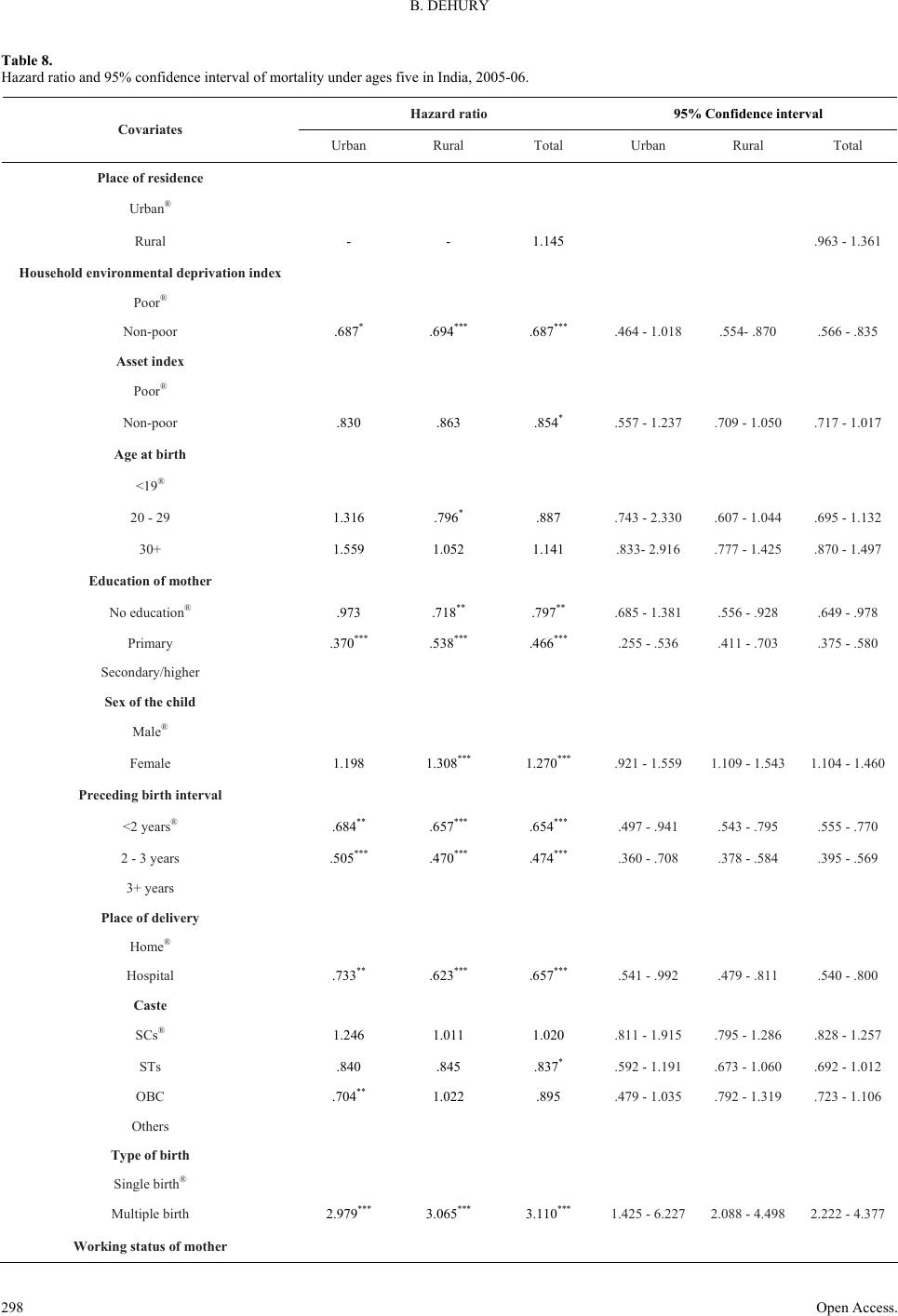
of mother and household environmental condition are signifi-
cant predictors of child survival. In rural India, age at birth,
education of mother, sex of child, preceding birth interval,
place of delivery, type of birth, duration of breastfeeding and
household environmental conditions are the significant predic-
tors of child survival.
Discussion and Conclusion
The study attempts to understand the association of house-
hold environmental conditions and asset index. Furthermore, it
attempts to understand the state of child survival by household
environmental conditions and asset index in India. Result shows
that the association of household environmental deprivation in-
dex and asset index is weaker and lower in rural areas than in ur-
ban areas. The association also varies among the states. In most
of the states the association between household environmental
deprivation index and asset index is low. Theoretically it is true
that the asset households tend to reside in good household en-
vironmental condition. However, the association between these
two indices in this study does not support the theoretical argu-
ment. We further found that there is no significant difference in
the risk of infant and child mortality among the asset poor and
those poor in household environmental deprivation index. In
most of the states, households living in poor household envi-
ronmental condition experienced higher mortality than the
households with poor asset status. The rural areas have rela-
tively higher risk of infant and under-five mortality than the ur-
ban areas. By analyzing the chance of child survival by indivi-
dual variables of household environmental condition, it is found
that the risk of infant and under-five mortality is lower among
the households having access to improved sources of drinking
water, flush toilet, and household using biogases as cooking
fuel and electrification. Hence these are found critical determi-
nants of child survival. The multivariate results show that along
with the socio-economic and demographic covariates, the house-
hold environmental deprivation is found a stronger predictor of
child survival. However, interestingly the relative hazard ratio
is higher in asset index compared to household environmental
deprivation index. It is also found that the hazard ratio is not a
significant predictor of child survival in rural and urban India.
It calls for improving the household environmental conditions
of the households in promoting child survival in India.
REFERENCES
Anderson, B. A., Romani, J. H., Phillips, H. E., & Zyl, J. A. V. (2002). En-
vironment, access to health care, and other factors affecting infant
and child survival among the African and colored populations of
South Africa, 1989-94. Population and E nvir on men t, 23, 349-364.
http://dx.doi.org/10.1023/A:1014530318272
Ayad, M., Barrere, B., & Otto, J. (1997). Demographic and socioecono-
mic characteristics of households. Demographic and Health Surveys,
26, Calverton, MD: Macro International.
Black, R. E., Cousens, S., Johnson, H. L., Lawn, J. E., Rudan, I., Bassa-
ni, D. G. et al. (2010). Global, regional, and national causes of child
mortality in 2008: A systematic analysis. Lan ce t , 375, 1969-1987.
http://dx.doi.org/10.1016/S0140-6736(10)60549-1
Boschi-Pinto, C., Velebitb, L., & Shibuya, K. (2008). Estimating child
mortality due to diarrhoea in developing countries. Bulletin of the
World Health Organization, 86, 710-717.
http://dx.doi.org/10.2471/BLT.07.050054
Cheng, J. J., Schuster-Wallace, C. J., Watt, S., Newbold, B. K., & Men-
te, A. (2012). An ecological quantification of the relationships be-
tween water, sanitation and infant, child, and maternal mortality. En-
vironmental Health, 11, 4.
http://dx.doi.org/10.1186/1476-069X-11-4
Fink, G., Gunther, I., & Hill, K. (2011). The effect of water and sanita-
tion on child health: evidence from the demographic and health sur-
veys 1986-2007. International Journal of Epidemiology, 40, 1196-
1204. http://dx.doi.org/10.1093/ije/dyr102
Folasade, I. B. (2000). Environmental factors, situation of women and
child mortality in south western Nigeria. Social Science & Medicine,
51, 1473-1489. http://dx.doi.org/10.1016/S0277-9536(00)00047-2
Hoque, B. A., Chakraborty, J., Chowdhury, J. T. A. et al. (1999). Ef-
fects of environmental factors on child survival in Bangladesh: A
case control study. Public Health, 113, 57-64.
International Institute for Population Sciences (IIPS) and Macro Inter-
national (2007). National Family Health Survey (NFHS III), 2005-06,
India. Mumbai: IIPS.
Kembo, J., & Ginneken, J. K. V. (2009). Determinants of infant and
child mortality in Zimbabwe: Results of multivariate hazard analysis.
Demographic Research, 21, 367-384.
http://dx.doi.org/10.4054/DemRes.2009.21.13
Lawn, J. E., Tinker, A., Mridha, M. K., & Anwar, I. (2006). Where is
maternal and child health now? Lancet, 368, 1474-1477.
http://dx.doi.org/10.4054/DemRes.2009.21.13
Mohanty, S. K. (2009). Alternative wealth indices and health estimates
in India. Genus, 2, 113-137.
Open Access 299
B. DEHURY
Muhuri, P. K. (1996). Estimating seasonality effects on child mortality
in Matlab, Bangladesh. Demography, 33, 98-110.
http://dx.doi.org/10.2307/2061716
Mutunga, C. J. (2007). Environmental determinants of child mortality
in Kenya. United Nations University. Research Paper No. 2007/83.
Pruss, A., Kay, D., Fewtrell, L., & Bartram, J. (2002). Estimating the
burden of disease from water, sanitation, and hygiene at a global
level. Environmental Health Perspective, 110, 537-542.
http://dx.doi.org/10.1289/ehp.02110537
Pruss-Ustun, A., Bos, R., Gore, F., & Bartram, J. (2008). Safer water,
better health: Costs, benefits and sustainability of interventions to pro-
tect and promote health. Geneva: World Health Organization.
Ram, F., Mohanty, S. K., & Ram, U. (2008). Progress and prospects of
millennium development goals in India. IIPS, Mumbai.
Sastry, N. (1996). Community based characteristics, individual and
household attributes, and child survival in Brazil. Demography, 33,
211-229. http://dx.doi.org/10.2307/2061873
Srivastava, A., & Mohanty, S. K. (2010). Economic proxies, household
consumption and Health estimates. Economic and Political Weekly,
16, 55-63.
WHO (2007). Indoor air pollution: National burden of disease esti-
mates.
You, D., Wardlaw, T., Salama, P., & Jones, G. (2010). Levels and trends
in under-5 mortality, 1990-2008. Lancet, 375, 100-103.
http://dx.doi.org/10.1016/S0140-6736(09)61601-9
Open Access.
300