Applied Mathematics, 2011, 2, 258-263
doi:10.4236/am.2011.22030 Published Online February 2011 (http://www.SciRP.org/journal/am)
The First Integral Method for Solving Maccari’s System
Davood Rostamy1,2, Fatemeh Zabihi1, Kobra Karimi1, Siamak Khalehoghli2
1Department of Mat hem at ic s, Imam Khomeini International University, Qazvin, Iran
2Department of Mat hem at ic s, Islamic Azad University, South Tehran Branch, Tehran, Iran
Received November 13, 2010; revised December 31, 2010; accepted January 4, 2011
Abstract
In this paper, we investigate the first integral method for solving the solutions of Maccari’s system. This idea
can obtain some exact solutions of this system based on the theory of Commutative algebra.
Keywords: First Integral Method, Maccari’s System, Exact Solution
1. Introduction
The first integral method was first proposed for solving
Burger-KdV equation [1] which is based on the ring
theory of commutative algebra. This method was further
developed by the same author in [2-10] and some other
mathematicians [2,11,12,13]. The present paper investi-
gates for the first time the applicability and effectiveness
of the first integral method on the Maccari’s. We consid-
er Maccari’s system:

2
=0,
=0.
txx
ty x
iQ QQR
RR Q






(1)
For the first time, Maccari derived this system from
the Kadomtsev-Petviash vili equ ation by using asymptoti-
cally exact reduction me t hod based Fo uri er expansi o n an d
spatiotemporal rescaling [14]. Maccari’s system is a kind
of nonlinear evolution equations that are often presented
to describe the motion of the isolated waves, localized in
a small part of space, in many fields such as hydrody-
namic, plasma physics, nonlinear optic, etc. Zhang used
Exp-function method for seeking exact solutions of
Maccari’s system [15].
The remaining structure of this article is organized as
follows: Section 2 is a brief introduction to the first in-
tegral method. In Section 3, implementing the first inte-
gral method, some new exact solutions for Maccari’s sy-
stem are reported. This describes ability and reliability of
the method. A conclusion and future directions for re-
search are all summarized in the last section.
2. The First Integral Method
Consider a general nonlinear PDE in the form


,,,,,,, ,,,,=0.
txyxxttyyxtxyytxxx
Puuu uuuuuuuu (2)
Using the wave variable =2
x
ykt

  carries in-
to the following ODE:


,, ,,=0,QUU UU

 (3)
where prime denotes the derivative with respect to the
same variable

.
Next, we introduce new independent variables =
x
u,
=yu

which change to a system of ODEs

=
=,.
xy
yfxy





 (4)
According to the qualitative theory of differential equ-
ations [1], if one can find two first integrals to system (4)
under the same conditions, then analytic solutions to (4)
can be solved directly. However, in general, it is difficult
to realize this even for a single first integral, because for a
given plane autonomous system, there is no general theo-
ry telling us how to find it’s first integrals in a systematic
way. A key idea of our approach here to find first inte-
gral is to utilize the division theorem. For convenience,
first let us recall the division theorem for two variables in
the complex domain  [4].
Theorem 2.1. Division theorem (see [14]) Suppose
that


,Pxy and


,Qxy are polynomials of two va-
riables x and y in


,
x
y and

,Pxy is irreducible
in


,
x
y. If


,Qxy vanishes at all zero points of


,Pxy, then there exists a polynomial


,Gxy in


,
x
y such that


,= ,,.QxyPxyGxy
3. Exact Solutions for Maccari’ s System
In order to seek exact solutions of system (1), we sup-

D. ROSTAMY ET AL.
259
pose

,,=,, exp,Qxytuxytikxytl  



 (5)
where ,k

and

are constants to be determined later,
l is an arbitrary constant. Substituting Equation (5) into
system (1) and yields




2
2
2=0,
=0,
txxx
ty x
iukuuku uR
RR u






(6)
Using the transformation
 
=, =, =2,uuRRxykt   (7)
where

is a constant, system (6) become the follow-
ing



2
2
=0,
2=0,
ukuuR
kR u


  





(8)
where prime denotes the differential with respect to

.
Integrating the second segment of Equation (8) with re-
spect to

and taking the integration constant as zero
yields yields
2
1
=.
2
Ru
k 

 (9)
Substituting Equation (9) into the first segment of (8)
yields

23
1=0.
2
uku u
k

  
 (10)
Next, we introduce new independent variables =
x
u,
=yu

which change Equation (10) to a system of ODEs

23
=
1
=.
2
xy
ykx x
k







(11)
Now, we are applying the Division Theorem to seek
the first integral to (9). Suppose that


=xx

and

=yy

are the nontrivial solutions to (9), and
 
=0
,= ,
mi
i
i
pxya xy

is an irreducible polynomial in


,
x
y such that
     
=0
,= =0,
mi
i
i
pxya xy  
 (12)
where
 
=0,1, ,
i
axi m are polynomials of x and
all relatively prime in


,
x
y,

0
m
ax. Equation
(10) is also called the first integral to (9). We start our
study by assuming =1m in (12). Note that dp
d

is a
polynomial in x and y, and
 
,=0px y  

implies

11
=0
dp
d

. By the Division Theorem, there exists a
polynomial






,=
H
xyhxgxy in


,
x
y such
that
 
 

   
11 11
11
1123
=0 =0
1
=0
=
1
=2
=,
ii
ii
ii
i
i
i
dpp xp y
dxy
axyiaxyk xx
k
hxgxya xy



  


 











(13)
where prime denotes differentiating with respect to the
variable x. On equating the coefficients of


=2,1,0
i
yi
on both sides of (13), we have




11
=,ax gxax
 (14)










010
=,axhxax gxax
 (15)


  
23
10
1=.
2
axk xxhxax
k







(16)
Since,


1
ax
is a polynomial of x, from (12) we con-
clude that


1
ax
is a constant and


=0.gx For sim-
plicity, we take


1=1ax , and balancing the degrees of


hx and


0
ax
we conclude that deg

=1hx , only.
Now suppose that


=hxAxB, then From (13), we
find

2
01
=,
2
axAx BxD
where D is an arbitrary integration constant. Substi-
tuting


0
ax
,


1
ax
and

hx in (14) and setting all
the coefficients of powers
x
to be zero, we obtain a
system of nonlinear algebraic equations and by solving it,
we obtain the following solutions:

2
22
=,=0,= 2,
2
2
A
BDk k
k



 (17)
and

2
22
=,=0,=2.
2
2
A
BDk k
k



 (18)
Using (15) and (16) in (10), we obtain

2
222
2=0,
2
22
kk
yx
k





and

2
222
2=0,
2
22
kk
yx
k





respectively. Combining this equations with (9), we ob-
tain the exact solutions of Equation (10) as follows:

D. ROSTAMY ET AL.
260

222
1 1
2
=2tanh 2,
2
ukk ikkkc
 

 




22 2
2 1
2
=2tanh 2,
2
ukk ikkkc
 

 



where 1
c is an arbitrary constant. Therefore, the exact solutions to (10) can be written as
 
22 2
1 1
2
,,=2tanh 22,
2
uxytkkik xyktkkc
 





 
22 2
2 1
2
,,=2tanh 22.
2
uxytkkikxyktkkc  

 



Then exact solutions for system (1) are




22 2
2
1 1
22 2
1 1
2
= 22,
tanh 2
2
=2tanh 22.
2
ikxyt l
Rk ikxyktkkc
Qe kk ikxyktkkc


 


 









(19)
and



22 2 2
2 1
22 2
2 1
2
= 22,
tanh 2
2
=2tanh (2)2.
2
ikxyt l
Rk ikxyktkkc
Qekkikx yktkkc


 







 




(20)
Now we assume that m = 2 in (10). By the Division
Theor em, there exists a polynomial
 
,=
H
xyhx gxy in


,
x
y such that
 
 

   
11 11
22
1123
=0 =0
2
=0
=
1
=2
=.
ii
ii
ii
i
i
i
dpp xp y
dxy
axyiaxyk xx
k
hxgxyaxy




 


 











(21)
On equating the coefficients of

=3,2,1,0
i
yi on
both sides of (21), we have

22
=,ax gxax
 (22)
 
121
=,axhxax gxax
 (23)
 


 
23
02
10
1
=2 2
,
ax axkxx
k
hxaxgxax








(24)


  
23
10
1=.
2
axk xxhxax
k







(25)
Since,

2
ax is a polynomial of x, from (20) we
conclude that

2
ax is a constant and

=0gx . For
simplicity, we take


2=1ax , and balancing the de-
grees of


,hx


0
ax and

1
ax we conclude that deg


=1hx or 0, therefore we have two cases:
Case1:
Suppose that deg


=1hx and

=hxAxB

, then
from (21) we f ind

2
11
=,
2
a xAxBxD
where D is an arbitrary integration constant. From (22)
we find
 


243
0
222
1
=82 22
12,
2
AAB
axx x
k
A
DBkx BDxE










 


where E is an arbitrary integration constant. Substituting


0
ax,


1
ax and


hx in (25) and setting all the co-
efficients of powers x to be zero, we obtain a system of
nonlinear algebraic equations and by solving it, we obtain





2
2
2
2
=,=0,
2
=22,
22
=,
2
kk
EB
Dkk
Ak






(26)

D. ROSTAMY ET AL.
261
and




2
2
2
2
=,
2
=0,
=22,
22
=.
2
kk
E
B
Dk k
Ak




 

(27)
Using (26) and (25) in (10), we obtain


2
22
1=0,
2
22
kk
yx
k





and


2
22
1=0,
2
22
kk
yx
k





respectively. Combining this Equations with (11), we
obtain two exact solutions to Equation (10) which was
obtained in case m = 1, i.e.

222
1 1
2
=2tanh 2,
2
ukkik kkc
 

 




22 2
2 1
2
=2tanh 2.
2
ukkik kkc
 

 



where 1 c is an arbitrary constant. Therefore, the exact solutions to (10) can be written as
 
22 2
1 1
2
,,=2tanh 22,
2
uxytkkikxyktkkc
 





 
22 2
2 1
2
,,=2tanh 22.
2
uxytkk ikxyktkkc  

 



Then the exact solutions for system (1) are:




22 2 2
1 1
22 2
1 1
2
= 22,
tanh 2
2
=2tanh22 .
2
ikxyt l
Rk ikxyktkkc
Qe kk ikxyktkkc


 


 









(28)
and




22 2 2
2 1
22 2
2 1
2
=22,
tanh2
2
=2tanh 22.
2
ikxytl
Rk ikxyktkkc
Qekkikx yktkkc


 


 




 




(29)
Case 2:
In this case suppose that deg

=0hx and

=hxA
, then from (21) we find

1=,ax AxB

where
B
is an arbitrar y integration constant. From (22)
we find
 

2
422
01
=,
22 2
A
axxkxABxD
k



 


where D is an arbitrary integration constant. Substi-
tuting

0
ax
,


1
ax
and


hx in (23) and setting all
the coefficients of powers x to be zero, we obtain a sys-
tem of nonlinear algebraic equations and by solving it,
we obtain =0, =0.AB (30)
Using (28) in (10), we obtain


2224
1=0.
22
ykx x
k
  
Combining this equations with (9), we obtain the exact
solutions to Equation (10) as follows:

22
1
22
1
22
2
32222
42 2
=,
4
ckk k
ckk k
kke
uee

 






 



22
1
22
1
22
2
422 22
42 2
=,
14
ckk k
ckk k
kke
u
e

 












where 1 c is an arbitrary constant. Then the exact solu-
tions to (10) can be written as: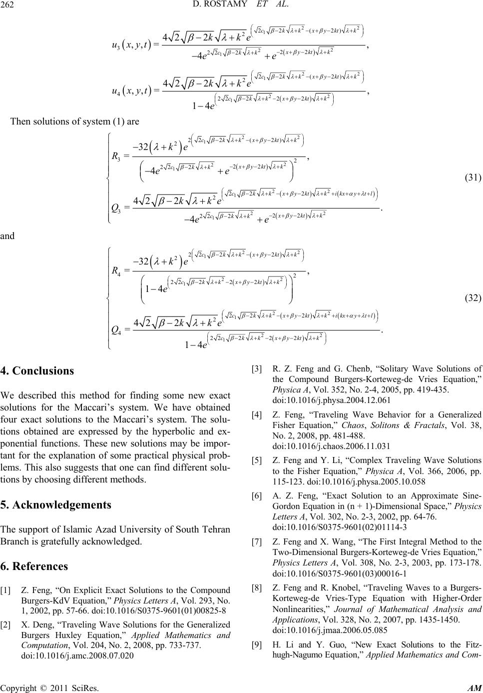

D. ROSTAMY ET AL.
262


22
1
2
2
1
22( 2)
2
322
22 2
42 2
,, =,
4
ckkxyktk
xykt k
ckk
kke
uxyt ee
 




 


 





22
1
22
1
22( 2)
2
422 222
42 2
,, =,
14
ckkxyktk
ckkxyktk
kke
uxyt
e
 
 


 



 




Then solutions of system (1) are




22
1
2 2
1
22
1
2
2
1
22 2(2)
2
32
22
222
222
2
322
22 2
32
=,
4
42 2
=.
4
ckkxyktk
xykt k
ckk
ckkxyktkikxytl
xykt k ckk
ke
R
ee
kke
Qee
 


 





 


 


 


 













(31)
and





22
1
22
1
22
1
22
1
22 22
2
42
22 222
222
2
422 222
32
=,
14
42 2
=.
14
ckkxyktk
ckkxyktk
ckkxyktkikxytl
ckkxyktk
ke
R
e
kke
Q
e
 
 
 
 



 



 



 



 














(32)
4. Conclusions
We described this method for finding some new exact
solutions for the Maccari’s system. We have obtained
four exact solutions to the Maccari’s system. The solu-
tions obtained are expressed by the hyperbolic and ex-
ponential functions. These new solutions may be impor-
tant for the explanation of some practical physical prob-
lems. This also suggests that one can find different solu-
tions by choosing different methods.
5. Acknowledgements
The support of Islamic Azad University of South Tehran
Branch is gratefully acknowledged.
6. References
[1] Z. Feng, “On Explicit Exact Solutions to the Compound
Burgers-KdV Equation,” Physics Letters A, Vol. 293, No.
1, 2002, pp. 57-66. doi:10.1016/S0375-9601(01)00825-8
[2] X. Deng, “Traveling Wave Solutions for the Generalized
Burgers Huxley Equation,” Applied Mathematics and
Computation, Vol. 204, No. 2, 2008, pp. 733-737.
doi:10.1016/j.amc.2008.07.020
[3] R. Z. Feng and G. Chenb, “Solitary Wave Solutions of
the Compound Burgers-Korteweg-de Vries Equation,”
Physica A, Vol. 352, No. 2-4, 2005, pp. 419-435.
doi:10.1016/j.physa.2004.12.061
[4] Z. Feng, “Traveling Wave Behavior for a Generalized
Fisher Equation,” Chaos, Solitons & Fractals, Vol. 38,
No. 2, 2008, pp. 481-488.
doi:10.1016/j.chaos.2006.11.031
[5] Z. Feng and Y. Li, “Complex Traveling Wave Solutions
to the Fisher Equation,” Physica A, Vol. 366, 2006, pp.
115-123. doi:10.1016/j.physa.2005.10.058
[6] A. Z. Feng, “Exact Solution to an Approximate Sine-
Gordon Equation in (n + 1)-Dimensional Space,” Physics
Letters A, Vol. 302, No. 2-3, 2002, pp. 64-76.
doi:10.1016/S0375-9601(02)01114-3
[7] Z. Feng and X. Wang, “The First Integral Method to the
Two-Dimensional Burgers-Korteweg-de Vries Equation,”
Physics Letters A, Vol. 308, No. 2-3, 2003, pp. 173-178.
doi:10.1016/S0375-9601(03)00016-1
[8] Z. Feng and R. Knobel, “Traveling Waves to a Burgers-
Korteweg-de Vries-Type Equation with Higher-Order
Nonlinearities,” Journal of Mathematical Analysis and
Applications, Vol. 328, No. 2, 2007, pp. 1435-1450.
doi:10.1016/j.jmaa.2006.05.085
[9] H. Li and Y. Guo, “New Exact Solutions to the Fitz-
hugh-Nagumo Equ a t i on , ” Applied Mathematics and Com-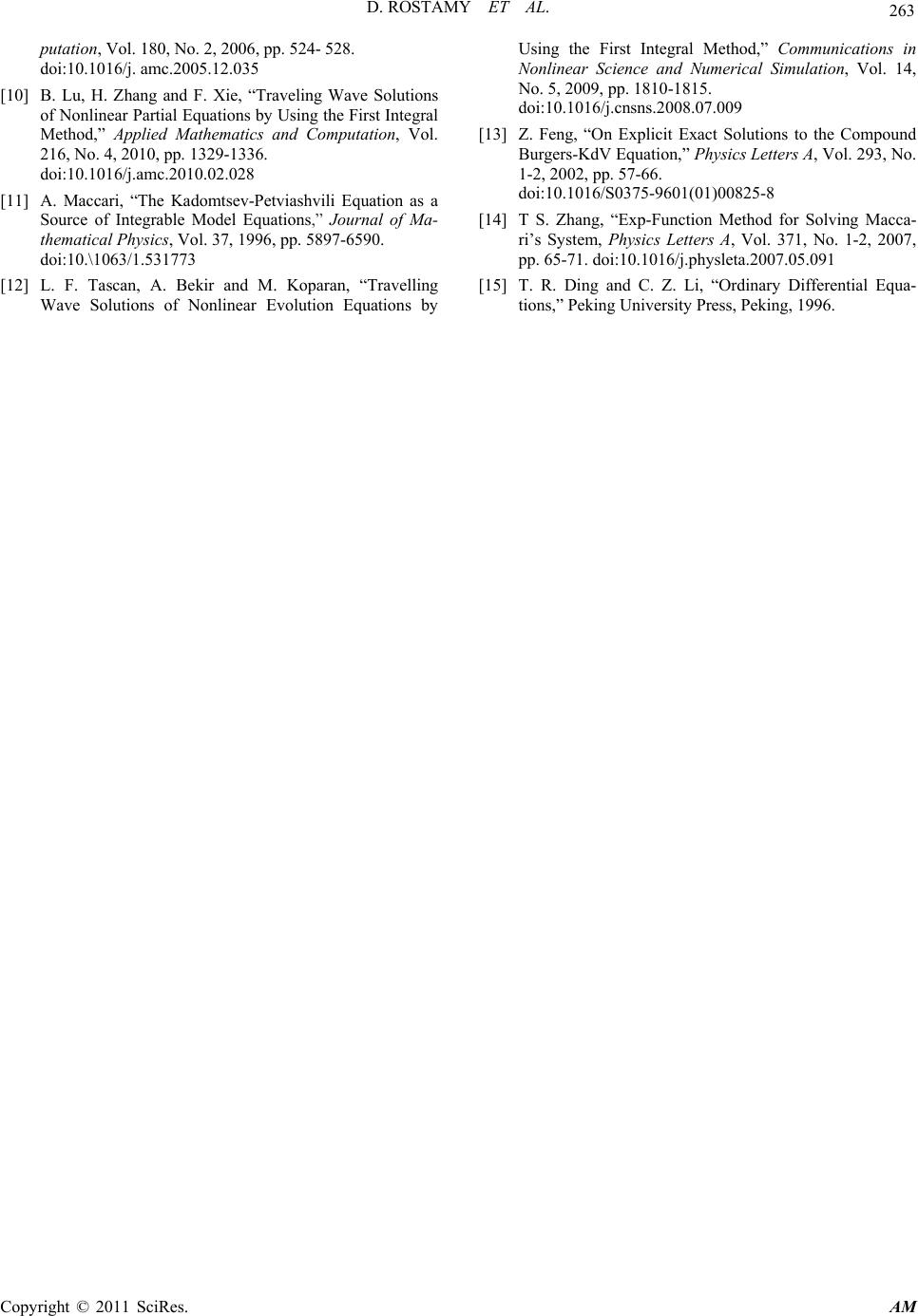

D. ROSTAMY ET AL.
263
putation, Vol. 180, No. 2, 2006, pp. 524- 528.
doi:10.1016/j. amc.2005.12.035
[10] B. Lu, H. Zhang and F. Xie, “Traveling Wave Solutions
of Nonlinear Partial Equations by Using the First Integral
Method,” Applied Mathematics and Computation, Vol.
216, No. 4, 2010, pp. 1329-1336.
doi:10.1016/j.amc.2010.02.028
[11] A. Maccari, “The Kadomtsev-Petviashvili Equation as a
Source of Integrable Model Equations,” Journal of Ma-
thematical Physics, Vol. 37, 1996, pp. 5897-6590.
doi:10.\1063/1.531773
[12] L. F. Tascan, A. Bekir and M. Koparan, “Travelling
Wave Solutions of Nonlinear Evolution Equations by
Using the First Integral Method,” Communications in
Nonlinear Science and Numerical Simulation, Vol. 14,
No. 5, 2009, pp. 1810-1815.
doi:10.1016/j.cnsns.2008.07.009
[13] Z. Feng, “On Explicit Exact Solutions to the Compound
Burgers-KdV Equation, ” Physics Lett ers A, Vol. 293, No.
1-2, 2002, pp. 57-66.
doi:10.1016/S0375-9601(01)00825-8
[14] T S. Zhang, “Exp-Function Method for Solving Macca-
ri’s System, Physics Letters A, Vol. 371, No. 1-2, 2007,
pp. 65-71. doi:10.1016/j.physleta.2007.05.091
[15] T. R. Ding and C. Z. Li, “Ordinary Differential Equa-
tions,” Peking University Press, Peking, 1996.