Paper Menu >>
Journal Menu >>
 Optics and Photonics Journal, 2013, 3, 351-359 Published Online November 2013 (http://www.scirp.org/journal/opj) http://dx.doi.org/10.4236/opj.2013.37055 Open Access OPJ Aplanatic and Telescopic Lens with a Radial Gradient of Refraction Index Vladimir Ivanovich Tarkhanov Joint stock Company “InfoTeCS”, Moscow, Russia Email: as174@yandex.ru Received September 12, 2013; revised October 9, 2013; accepted October 29, 2013 Copyright © 2013 Vladimir Ivanovich Tarkhanov. This is an open access article distributed under the Creative Commons Attribution License, which permits unrestricted use, distribution, and reproduction in any medium, provided the original work is properly cited. ABSTRACT It is shown that aplanatic lens with a radial gradient of refraction index is simultaneously a telescopic lens, notably not only for an axial beam, but also for an off axis parallel beam. Consideration is carried out by an algebraic way on the basis of regularities of ray paths. It is also shown that aplanatic and telescopic properties of the lens are independent of the refracting surface shapes. Various versions of lens performance are shown below. Keywords: Aplanatic Lens; Telescopic Lens; Radial Gradient; Refraction Index 1. Introduction Aplanatic lenses with an axial and radial gradient of the refraction index are known by now. In these lenses, spherical aberration for a point on the optical axis is strictly eliminated. Earlier possibility of creation of an aplanatic lens with an axial gradient of the refractive index was shown [1]. The homocentric beam leaving a point of 1 M on an optical axis, reaches to the first surface of a lens, refracts on it and then propagates parallel to an optical axis in the lens medium. Then, refracting on the second surface of a lens, the rays of the beam forms a homocentric dispers- ing beam again (Figure 1). Virtual continuations of the ray forms the virtual image at the axial point 2 M on the optical axis. Various gra- dients of the refractive index and the related refracting surfaces can be used for formation of a lens. The calcula- tions for lens parameters were provided with spherical and parabolic surfaces of revolution. An aplanatic gradient lens [2] limited by the first and the second refracting surfaces of revolution with thickness by the axis , which is multiple of double nominal focal length, made of a material with a radial distribution of the refraction index determined from the equa- tion dz ny 00 sech 2expexpny naynayay , (1) where 0 is the refraction index value on the axis; is the constant; having generatrix n a 1 y z of the 1st convex surface defined by the equation: 22 2 112 1 F yzny zsny z , (2) where F s is the front distance; and having generatrix 2 y z of the 2nd concave surface defined by the equa- tion: 2 22 2121 F yzny zdsnyzd , (3) where F s is the rare distance; hence, F F s s . The shape of both refracting surfaces in the known lens is equal. Generatrixes of Equation (2) and Equation (3) may be conditionally called hyperbolas of the higher or- der. It is known that the pitch (periodicity length) for the refractive index (RI) distribution is determined by the Еquation (1) and also called the hypersecans one equals [3] L 2πLa , as a consequence, the half of the periodicity length is 2πLa The nominal focal length of the lens with hypersecans RI distribution is 04π2 f La , double nominal focal length will be equal to half the pe- riodicity length 0 22π F fL a  V. I. TARKHANOV 352 Figure 1. The known aplanatic lens with axial gradient. When selecting certain thickness of the lens with the RI distribution of type Equation (1) and flat 1st and 2nd sur- faces normal to the optical axis, focusing, diverging or telescopic lens can be obtained [3]. Hence, it is quite ob- vious that the telescopic lens is obtained in the case of selecting the thickness of the lens equal to twice the nominal focal length. As a result, the input parallel beam of rays, which is also parallel to the optical axis, becomes strictly parallel when leaving the lens. The ray path equation in the medium with RI distribu- tion Equation (1) is also known. For instance, if the initial height of a point, from which the ray is initiated, equals C, the initial coordinate is C, and the initial direction coefficient (the initial ray tangent) 1 b z is , then the ray path equation becomes as follows [4] 1 1arshshcoshsin R CCC yz abaz zcabaz z a C (4) As a consequence, considering that 2 arsh ln1xxx and 2 arsh 11xx one can write down that 1 shcosh sin CCCC x abaz zcabaz z , 2 ln 1 R y zxxa , and the derivative is obtained from the expression 1 2 1 h cossh sin sh coshsin1 R CCCC CCCC yz cabazzabaz z abaz zcabazz (5) Note that if the length between the coordinates of the ray exits point from the lens Е z and the ray entrance point of the lens D z E D dz z equals to the periodicity length 2πLa , then according to Equation (4) the height of ray exit point from the lens E y is equal to the height of ray entrance point to the lens D y, or E D yy (6) As a result, the RI value at the ray entrance point to the lens will be equal to the RI value at the ray exit point from the lens E D ny ny (7) In this case, according to Equation (5), the ray tangent 2 occurring in the ray exit point from the lens before the refraction will equal to the initial tangent 1 21 (8) and the derivative will correspond to the initial one R DRE y zyz (9) If the length between coordinates of the ray exit point from the lens d E z and coordinates of the ray en- trance point to the lens D z equals to the half periodicity length, 2πLa , then according to Equation (4) the height of the ray exit point from the lens E y will be equal to the height of the ray entrance point to the lens D y with the sign reversed E D yy (10) The RI value at the ray entrance point to the lens will be equal to that at the ray exit point from the lens E D ny ny The ray tangent 2 occurring at the ray exit point from the lens before the refraction will be equal to the initial tangent 1 with the sign reversed 21 (11) The value of derivative will be equal in the absolute magnitude to the initial one taken with the sign reversed R DRE y zyz (12) According to the design, in the known aplanatic lens, every ray of the homocentric radiation beam exiting from a point on the optical axis, after the refraction on the 1st surface becomes parallel to the optical axis. Then spread- ing inside the lens, in a gradient medium by a curvilinear symmetrical path, each ray reaches the 2nd refractive sur- face. In the cross-point with the 2nd refractive surface the ray is also parallel to the optical axis. After the refraction on the 2nd surface, each ray obtains the initial direction which allows re-forming a homocen- Open Access OPJ  V. I. TARKHANOV 353 tric diverging beam with the center located on the optical axis, at a distance of F F s s from the 2nd surface cen- ter. Hence, F s is the rear distance (Figure 2). Depending on the selected thickness of the lens, which is multiple to the double nominal focal length, the refraction on the 2nd surface may happen both above and below the axis (if we conditionally assume the initial re- fraction on the 1st surface occurring above the optical axis). Thus, however causes no effect on the lens ability to form a homocentric diverging beam at the exit (Figure 3). d The known lens allows formation of a homocentric di- verging radiation beam at the exit with the only help of two refractive surfaces of revolution of the same shape, which generatrix is rather complicated, Equation (2) and Equation (3), that makes its manufacture rather complex. Thus, the fact that the other surfaces, including one simpler shape, cannot be used as the refractive surfaces is the disadvantage of the known lens restricting possibili- ties of its manufacture. 2. Analytical Treatment Disadvantages of the known lens can be avoided, if we consider a remarkable, previously unknown property of the primary lens, which has a thickness multiple to the periodicity length, to preserve initial direction of the ray at the exit point, which appears on the 1st surface, inde- pendently of a chosen shape of the 1st and the 2nd sur- faces, as well as front distance value and location of the radiation source, respectively. The lens having a thickness multiple to half the perio- dicity length possesses a similar property of preserving the absolute value of the direction coefficient at the exit point for the entrance ray appearing on the 1st surface, Figure 2. The known aplanatic lens with thickness . L Figure 3. The known aplanatic lens with thickness 2L. independently of the shapes selected for the 1st and 2nd surfaces, as well as of the front distance and location of the source of radiation, respectively. However, in this case the direction coefficient sign at the exit point for the refracted ray reverses. Let us show the effect of these properties, firstly for the lenses of the minimal thickness with the thickness equal to the periodicity length and half periodicity length L 2L. For the lenses of a greater thickness multiple to half the periodicity length, these properties also take effect. A lens of thickness , by the optical axis at a distance equal to the periodicity length is made from a mate- rial with the radial RI distribution d L ny , which corre- sponds to (1) and is known for the given wavelength, and is limited by the refracting 1st and 2nd surfaces of the same shape with generatrixes 1 y z and 2 y z and disposed in a homogeneous medium (assume homogene- ous medium RI 1 1n (air)). In the case under consideration, the same shape of the refracting surfaces of the lens thickness, which is equal to the periodicity length , means that the 2nd surface represents the 1st surface after parallel translation along the optical axis by a distance . d L z d As a result, a distance along the axis between any separate initial point on the 1st surface, which has a cer- tain height above the axis , and a point on the 2nd sur- face having the same height above the axis and lo- cated on a straight line parallel to the axis with the initial point of the 1st surface will be the same and equal to the thickness z z z z dL . In the simplest case, the refracting 1st and 2nd surfaces of the same shape may be the surfaces of revolution, but in more general case, this is optional. The 1st surface vertex is located in the origin of the co- ordinate system. The axis represents the optical axis of the lens. Assuming that the lens is axially symmetrical, consideration is made in the meridional plane. z The incident beam for the 1st surface originating from the point 1 M of the optical axis has a direction coeffi- cient 1К1 u and is refracted in the point A having coordinates 1C, 1C. Let us denote: the angle of inci- dence of a ray on the 1st surface as 1 z y , the angle of re- fraction on the 1st surface as 1 , normal to the 1st sur- face in a point A as , the angle of incidence of a ray on the 2nd surface as 2 1 N , the angle of refraction on the 2nd surface as 2 , and normal to the 2nd surface in a point B as . 2 Let us denote: direction coefficient of the entrance ray refracting on the 1st surface in point A as 1T, direction coefficient of the ray refracted on the 1st surface in a point A as 1 N u E u, direction coefficient of the ray refracting on the 2nd surface in a point B as , and direction co- 2T u Open Access OPJ  V. I. TARKHANOV 354 efficient of the ray refracted on the 2nd surface in a point B as 2 E u. Direction coefficient 1 N u of the normal 1 to the 1st surface in a point A can be expressed as follows: N 11 1 N uy z, (13) where 1 y z is the 1st derivative of 1 y z. Direction coefficient 2 N u of the normal 2 to the 2nd surface in a point B can be expressed as follows: N 22 1 N uyz , (14) where 2 y z is the 1st derivative of 2 y z. Let us consider the case of the 1st convex and the 2nd concave surfaces for a lens with the thickness multiple to ( Figure 4). L The refraction scheme in Figure 3 relates to cases when after the refraction the direction coefficient 1 E u of the exit ray refracted on the 1st surface is negative. For this case, a general scheme of the ray path in the lens is shown in Figure 5. For the refraction schemes shown in Figure 3, the an- gle of incidence 1 in the point A on the 1st surface can be determined from the following expression: 111 1 tan 1 TN TN uu uu 1 , (15) and the angle of refraction 1 is obtained from the ex- pression 111 1 tan 1 EN EN uu uu 1 1 , (16) Moreover, according to Snell's refraction law 11 1 sin sin C nny , where is the RI in the refraction point A. C1 ny Then, with regard to the fact that , the refraction angle is expressed as 11n 11C sinsin ny 1 (17) Figure 4. Schemes of refraction on the 1st convex and the 2nd concave surfaces for a lens with the thickness multiple to . L Figure 5. The ray path scheme for the lens with the thick- ness multiple to , having the 1st convex and the 2nd con- cave surfaces. L Since the ray refracted in the point A on the 1st surface, which has the initial direction 1 E u, spreads after the re- fraction by a curvilinear path with a period equal to the periodicity length , then in the point B, after complet- ing the full period: L 1) according to the condition Equation (6), the height of the refraction point B will be equal to the height of the refraction point A; 2C y C y1 2) according to the condition Equation (8), direction coefficient 22T u of the ray incident to the 2nd sur- face will be equal to 1E u1 and, respectively, 2T uu1E ; (18) 3) according to the condition Equation (8) and ratios Equation (9), Equation (13) and Equation (14), and since shapes of the 1st and 2nd surfaces are the same, direction coefficient 2 N u of the normal 2 to the 2nd surface in the point B will be equal to the direction coefficient 1 N N u of the normal to the 1st surface in the point A, and thus 1 N 21 N N uu (19) The angle of incidence 2 in the point B will be equal to 222 2 tan 1 TN TN uu uu 2 (20) Taking into account Equation (18) and Equation (19) and substituting them into Equation (20), we get: 2111 tan 1 EN EN uu uu 1 (21) Comparing Equation (16) and Equation (21), we get: 12 On this basis, we can write down that 2 sinsin1 (22) For the point B on the 2nd surface, according to Snell's refraction law, C22 12 sin sinny n , where C2 ny is the RI on the refraction point B. Considering that 11n , the angle of refraction will be as follows: 22 sin sin C ny 2 Taking into consideration relations Equation (17) and Equation (22), we get: 221 sin sin CC ny ny 1 C Since 21C yy in the point B, as mentioned above, and according to Equation (7), respectively, the expres- sion 2C ny ny1C is true, and we get: 21 sin sin Then, as a consequence, Open Access OPJ 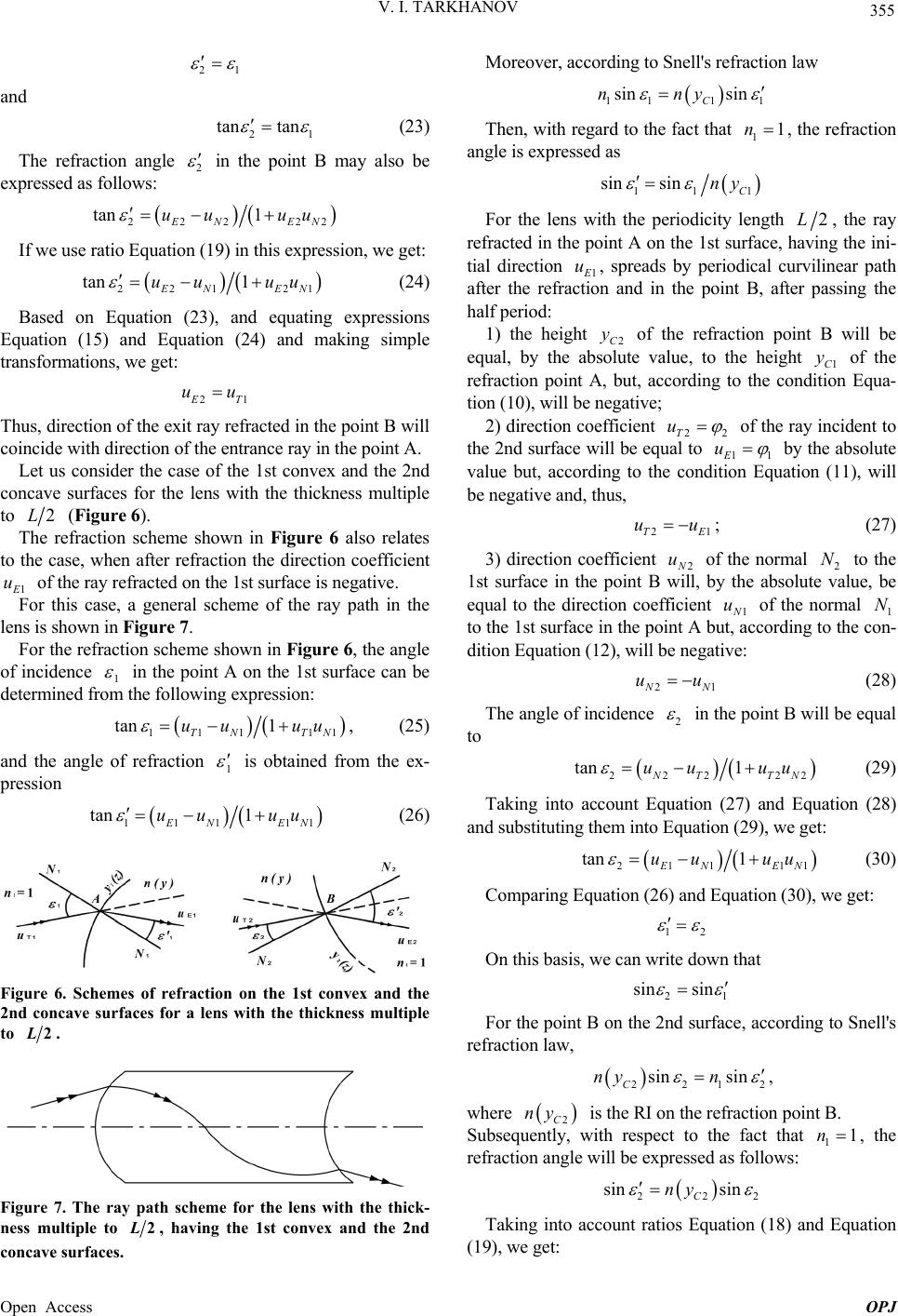 V. I. TARKHANOV 355 21 and 21 tan tan (23) The refraction angle 2 in the point ex B may also be pressed as follows: 2 tan uu 22 22 1 EN EN uu If we use ratio Equation (19) in this expression, we get: 221 21 tan 1 EN EN uu uu (24) Based on Equation (23), and equatin Eq g expressions uation (15) and Equation (24) and making simple transformations, we get: 21 E T uu Thus, direction of the exit ray refracted in the point B will coincide with direction of the entrance ray in the point A. Let us consider the case of the 1st convex and the 2nd concave surfaces for the lens with the thickness multiple to 2L (Figure 6). The refraction scheme shown in Figure 6 also relates to the case, when after refraction the direction coefficient 1 E u of the ray refracted on the 1st surface is negative. For this case, a general scheme of the ray path in the lens is shown in Figure 7. For the refraction scheme shown in Figure 6, the angle of incidence 1 in the point A on the 1st surface can be determined from the following expression: 111 1 tan 1 TN T uu uu 1N , (25) and the angle of refraction 1 is obtained fr om the ex- pression 111 1 tan 1 EN EN uu uu 1 (26) Figure 6. Schemes of refraction on the 1st convex and the 2nd concave surfaces for a lens with the thickness multiple to 2L. Figure 7. The ray path scheme for the lens with the thick ness multiple to- 2L, having the 1st convex and the 2nd concave surfaces. 1 Moreover, according to Snell's refraction law 11 1 sin sin C nny Then, with regard to the fact that 11n, the refraction angle is expressed as 11 sin sinC ny For the lens with t 1 he periodicity length 2L, the ray refracted in the point A on the 1st surface, having the ini- tial direction 1 E u, spreads by periodical curvilinear path af ht int t, according to the condition Equa- tio ter the refraction and in the point B, after passing the half period: 1) the heig2C y of the refraction point B will be equal, by the absolute value, to the height 1C y of the refraction po A, bu n (10), will be negative; 2) direction coefficient 22T u of the ray ident to the 2nd surface will be equal to 11E u inc by the absolute value but, according to the condition Equation (11), will be negative and, thus, 21TE uu ; (27) 3) direction coefficie2 N u nt of the normal to the 1st surface in the point B will, b equal to the direction coefficient 2 N y the absolute value, be 1 N u of the normal N 1 but, according the con- dition Equation (12), will be negative: 21 to the 1st surface in the point Ao t N N uu (28) The angle of incidence 2 in the point B will be equal to 22222 tan 1 NT TN uu uu (29) Taking into account Equation (27) and Equation (28) and substituting them into Equation (29), we get: 211 11 tan 1 EN EN uu uu (30) Comparing Equation (26) and Equation (30), we get: 12 On this basis, we can write down that 21 sin sin For the point B on the 2nd surface, according to Snell's refraction law, 2212 sin sin C ny n , where 2C ny is the RI on the refraction point B. Subseq, with respect to the fact that uently 1 1n , the refraction angle will be expressed as follows: 222 sin sin C ny Taking into account ratios Equation (18) an d Equation (19), we get: Open Access OPJ 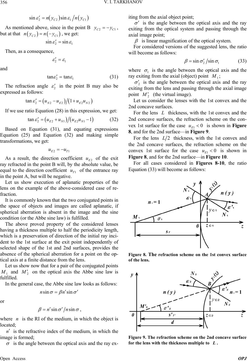 V. I. TARKHANOV 356 221 sin sin CC ny ny 1 As mentioned above, since in the point B 21CC yy , but at that n 21CC yn y , we get: 21 sin sin Then, as a consequence, 12 and 21 tan tan (31) The refraction angle 2 in the point B may also be ssed as follows: expre 222 22EN uu tan 1 NE uu ( If we use ratio Equation28) in this expression, we get: 22121 tan 1 EN EN uu uu (32) Based on Equation (31), and equating expressions Eq transformations, we get: uation (25) and Equation (32) and making simple 21 E T As a result, the direction coefficient 2 uu E u of the exit ray refracted in the point B will, by the absolute value, be equal to the direction coefficient 1T u e of the entrance ray in the point A, but will be negativ th pendently of se . Let us show execution of aplanatic properties of the lens on the example of the above-considered case of re- fraction. It is commonly known that the two conjugated points in e space of objects and images are called aplanatic, if spherical aberration is absent in the image and the sine condition (or the Abbe sine law) is fulfilled. The above proved property of the considered lenses having a thickness multiple to half the periodicity length, which is a preservation of direction of the initial ray inci- dent to the 1st surface at the exit point inde lected shape of the 1st and 2nd surfaces, provides the absence of the spherical aberration for a point on the op- tical axis at a finite distance from the lens. Let us show now that for a pair of the conjugated points 1 M and 2 M on the optical axis the Abbe sine law is fulfilled. In the general case, the Abbe sine law looks as follows: sin sinnn or sin sinnn , where is the RI of the medium, in which the object is ted; is the refractive index of the meum, in which the image is formed; n loca n di iting from the axial object point; is the angle between the optical axis and the ray exiting from the optical system and passing through the axial image point; is linear magnification of the optical system. For considered versions of the suggested lens, the ratio will become as follows: 21 sin sin (33) where 1 is the angle between the optical axis and the ray exiting from the axial (object) point 1 M ; 2 is the angle between the optical axis and the ray exiting from the lens and passing through the axial image point 2 M (the virtual image). Fo is shown in Fi gure 8, Let us consider the lenses with the 1st convex and the 2nd concave surfaces. r the lens L thickness, with the 1st convex and the 2nd concave surfaces, the refraction scheme on the con- vex 1st surface for the case 1E u0 and for the 2nd surface—in Figure 9. For the lens 2L thickness, with the 1st convex and the 8-10, the ratio Eq e 2nd concavsurfaces, the refraction scheme on the convex 1st surface for the case 10 E u is shown in Figure 8, and for the 2nd surface—in Figure 10. For all cases considered in Figures uation (33) will become as follows: Figure 8. The refraction scheme on the 1st convex surface of the lens. Figure 9. The refraction scheme on the 2nd concave surface for the lens with the thickness multiple to L. is the angle between the optical axis and the ray ex- Open Access OPJ 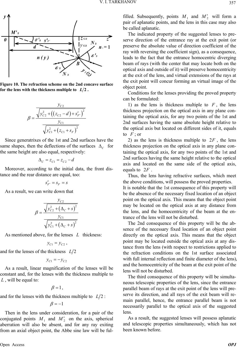 V. I. TARKHANOV 357 Figure 10. The refraction scheme on the 2nd concave surface for the lens with the thickness multiple to 2L. 2 2 2 22 1 2 2 11 C CCF C CCF y yzds y yzs Since generatrixes of the 1st and 2nd surfaces have the same shapes, then the deflections of the surfaces C for the same height are also equal, respectively: Moreover, according to the initial data, the front dis- 12CC C zzd tance and the rear distance are equal, too: FF s ss As a result, we can write down that 2 2 2 C y ys As mentioned above, for the lenses thickness: 2 1 2 2 1 CC C CC y ys L 12CC yy, and for the lenses of the thickness 2L 12CC As a result, linear magnification of yy the lenses will be constant and, for the lenses with the thickness multiple to , will be equal to: L 1 , and for the lenses with the thickness multiple to 2L: 1 Then in the lens under consideration, for a pair of the conjugated points 1 M and 2 M on the axis, spherical d fny ray exiting from an axial object point, the Abbe sine law will be ful- filled. Subsequently, points aberration will also be absent, anor a 1 M and 2 M direction coefficient of the y locat iple to will form a pa see entrance ray at the exit point (or preserve the absolute value of equce, beam of rays (with the center mae both on the op iding the pr thicult ir of aplanatic points, and the lens in this case may also be called aplanatic. The indicated property of the suggested lenses to pre- rve direction of th ray with reversing the coefficient sign), as a consen leads to the fact that the entrance homocentric diverging tha ov kness m t tical axis and outside of it) will preserve homocentricity at the exit of the lens, and virtual extensions of the rays at the exit point will concur forming an virtual image of the object point. Conditions for the lenses proved property can be formulated: 1) as the lens is F , the lens thickness projection on the optical axis in any plane con- taining the optical axis, for any two points of the 1st and 2nd surfaces having the same absolute height relative to the optical axis but located on different sides of it, equals to F ; or 2) as the lens is thickness multiple to 2 F , the lens thickness projection on the optical axis in any plane con- taining the optical axis, for any two points of the 1st and 2nd surfaces having the same height relative to the optical axis and located on the sa eq me side of the optical axis, uals to 2 F . Thus, the lens having refractive surfaces, which meet th lend the homocentricit at the en- tra the lens (with respect to restrictions applied to th ), beam will re- m e above conditions, will possess the proved properties. It is notable that the 1st consequence of this property will be the absence of the necessary fixed location of an object point on the optical axis. This means that the object point may be located on the optical axis at any distance from thens, ay of the beam xit nce of the lens will not be disturbed. The 2nd consequence of this property will be the ab- sence of the necessary fixed location of an object point directly on the optical axis. This means that the object point may be located outside the optical axis at any dis- tance from e refraction conditions on the 1st surface associated with full internal reflection and finite diameter of the lens and the homocentricity of the beam at the exit point of the lens will not be disturbed. The third consequence of this property will be simulta- neous telescopic properties of the lens, since the entrance parallel beam of rays at the exit point of the lens will pre- serve its direction, and all rays of the e ain parallel, hence, the entrance parallel beam is not necessarily parallel to the optical axis of the suggested lens. As a result, the suggested lenses will possess aplanatic and telescopic properties simultaneously, which has not been known before. Open Access OPJ 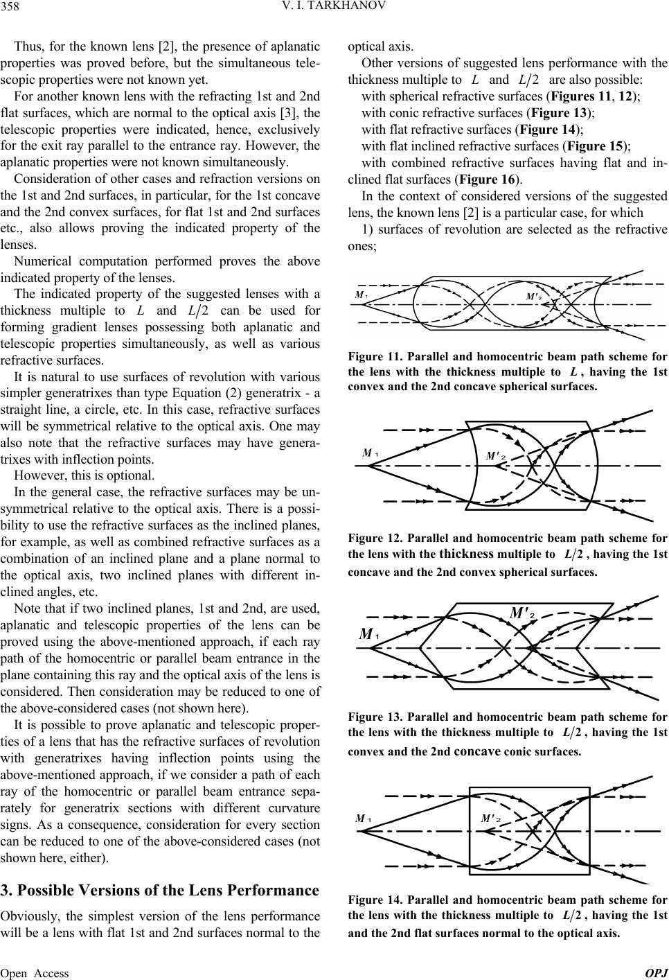 V. I. TARKHANOV 358 Thus, for the known lens [2], the presence of aplanatic properties was proved before, but the simultaneous tele- scopic properties were not known yet. t and 2nd surfaces, in particular, for the 1st concave an sted lenses with a th For another known lens with the refracting 1st and 2nd flat surfaces, which are normal to the optical axis [3], the telescopic properties were indicated, hence, exclusively for the exit ray parallel to the entrance ray. However, the aplanatic properties were not known simultaneously. Consideration of other cases and refraction versions on the 1s d the 2nd convex surfaces, for flat 1st and 2nd surfaces etc., also allows proving the indicated property of the lenses. Numerical computation performed proves the above indicated property of the lenses. The indicated property of the sugge ickness multiple to L and 2L can be used for forming gradient lenses possessing both aplanatic and telescopic properties simultaneously, as well as various refractive surfaces. It is natural to use surfaces of revolution with various si ith inflection points. tive surfaces may be un- sy o inclined planes with different in- cl the optical axis of the lens is co ay be reduced to one of th rix sections with different curvature si rmal to the op mpler generatrixes than type Equation (2) generatrix - a straight line, a circle, etc. In this case, refractive surfaces will be symmetrical relative to the optical axis. One may also note that the refractive surfaces may have genera- trixes w However, this is optional. In the general case, the refrac mmetrical relative to the optical axis. There is a possi- bility to use the refractive surfaces as the inclined planes, for example, as well as combined refractive surfaces as a combination of an inclined plane and a plane normal to the optical axis, tw ined angles, etc. Note that if two inclined planes, 1st and 2nd, are used, aplanatic and telescopic properties of the lens can be proved using the above-mentioned approach, if each ray path of the homocentric or parallel beam entrance in the plane containing this ray and nsidered. Then consideration m e above-considered cases (not shown here). It is possible to prove aplanatic and telescopic proper- ties of a lens that has the refractive surfaces of revolution with generatrixes having inflection points using the above-mentioned approach, if we consider a path of each ray of the homocentric or parallel beam entrance sepa- rately for generat gns. As a consequence, consideration for every section can be reduced to one of the above-considered cases (not shown here, either). 3. Possible Versions of the Lens Performance Obviously, the simplest version of the lens performance will be a lens with flat 1st and 2nd surfaces no tical axis. Other versions of suggested lens performance with the thickness multiple to L and 2L are also possible: with spherical refractive surfaces (Figures 11, 12); with conic refractive surfaces (Figure 13); with flat refractive surfaces (Figure 14); with flat inclined refractive surfaces (Figure 15); with combined refractive surfaces having flat and in- clined flat surfaces (Figure 16). In the context of considered versions of the suggested lens, the known lens [2] is a particular case, for which 1) surfaces of revolution are selected as the refractive ones; Fith scheme for th e 1st co gure 11. Parallel and homocentric beam pa e lens with the thickness multiple to L, having th nvex and the 2nd concave spherical surfaces. Figure 12. Parallel and homocentric beam path scheme for the lens with the thickness multiple to 2L, having the 1st concave and the 2nd convex spherical surfaces. Figure 13. Parallel and homocentric beam path scheme for the lens with the thickness multiple to 2L, having the 1st convex and the 2nd concave conic surfaces. Figure 14. Parallel and homocentric beam path scheme for the lens with the thickness multiple to 2L, having the 1st and the 2nd flat surfaces normal to the optical axis. Open Access OPJ 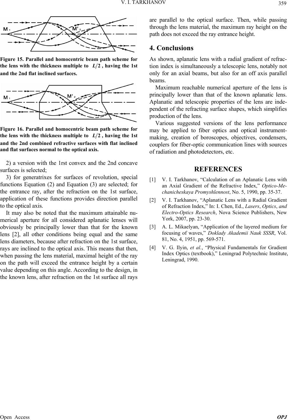 V. I. TARKHANOV Open Access OPJ 359 Figure 15. Parallel and homocentric beam path scheme for the lens with the thickness multiple to 2L, having the 1st and the 2nd flat inclined surfaces. Figure 16. Parallel and homocentric beam path scheme for the lens with the thickness multiple to 2L wit , having the 1st and the 2nd combined refractive surfacesh flat inclined and flat surfaces normal to the optical axis. d t s of revolution, special functions Equation (2) and Equation (3) are selected; for the entrance ray, after the refraction on the 1st surface, application of these functions provides direction parallel to the optical axis. It may also be noted that the maximum attainable nu- merical aperture for all considered aplanatic lenses will qua eans that then, hen passing the lens material, maximal height of the ray on his angle. According to the design, in th lanatic lens. copic properties of the lens are inde- cting surface shapes, which simplifies creation of boroscopes, objectives, condensers, co [1] ience Publishers, New York, 2007, pp. 23-30. [3] A. L. Mikaelyyered medium for are parallel to the optical surface. Then, while passing through the lens material, the maximum ray height on the path does not exceed the ray entrance height. 4. Conclusions As shown, aplanatic lens with a radial gradient of refrac- tion index is simultaneously a telescopic lens, notably not only for an axial beams, but also for an off axis parallel beams. Maximum reachable numerical aperture of the lens is principally lower than that of the known ap Aplanatic and teles pendent of the refra production of the lens. Various suggested versions of the lens performance may be applied to fiber optics and optical instrument- making, uplers for fiber-optic communication lines with sources of radiation and photodetectors, etc. REFERENCES 2) a version with the 1rst convex anhe 2nd concave surfaces is selected; 3) for generatrixes for surface V. I. Tarkhanov, “Calculation of an Aplanatic Lens with an Axial Gradient of the Refractive Index,” Optico-Me- chanicheskaya Promyshlennost, No. 5, 1990, pp. 35-37. [2] V. I. Tarkhanov, “Aplanatic Lens with a Radial Gradient of Refraction Index,” In: I. Chen, Ed., Lasers, Optics, and Electro-Optics Research, Nova Sc obviously be principally lower than that for the known lens [2], all other conditions being el and the same lens diameters, because after refraction on the 1st surface, rays are inclined to the optical axis. This m an, “Application of the la foc Ind using of waves,” Doklady Akademii Nauk SSSR, Vol. 81, No. 4, 1951, pp. 569-571. [4] V. G. Ilyin, et al., “Physical Fundamentals for Gradient ex Optics (textbook),” Leningrad Polytechnic Institute, Leningrad, 1990. w the path will exceed the entrance height by a certain value depending on t e known lens, after refraction on the 1st surface all rays |