Applied Mathematics, 2011, 2, 247-253
doi:10.4236/am.2011.22028 Published Online February 2011 (http://www.SciRP.org/journal/am)
Matrix Padé-Type Method for Computing the Matrix
Exponential
Chunjing Li1, Xiaojing Zhu1, Chuanqing Gu2
1Department of Mat hem at ic s, Tongji University, Shanghai, China
2Department of Mat hem at ic s, Shanghai University, Shanghai, China
Received October 31, 2010; revised December 23, 2010; accepted December 28, 2010
Abstract
Matrix Padé approximation is a widely used method for computing matrix functions. In this paper, we apply
matrix Padé-type approximation instead of typical Padé approximation to computing the matrix exponential.
In our approach the scaling and squaring method is also used to make the approximant more accurate. We
present two algorithms for computing
A
e and for computing
A
t
e with many 0t respectively. Numeri-
cal experiments comparing the proposed method with other existing methods which are MATLAB’s func-
tions expm and funm show that our approach is also very effective and reliable for computing the matrix ex-
ponential
A
e. Moreover, there are two main advantages of our approach. One is that there is no inverse of a
matrix required in this method. The other is that this method is more convenient when computing
A
t
e for a
fixed matrix A with many 0t.
Keywords: Matrix PadÉ-Type Approximation, Matrix Exponential, Scaling and Squaring, Backward Error
1. Introduction
The matrix exponential is the most studied and the most
widely used matrix function. It plays a fundamental role
in the solution of differential equations in many applica-
tion problems such as nuclear magnetic resonance spec-
troscopy, Markov models, and Control theory. These
problems often require the computation of At e for a
fixed matrix and many 0t
For example, with some suitable assumptions on the
smooth of a function
f
, the solution to the inhomoge-
neous system

,,0 ,,,
nnn
dy Ayftyyc yA
dt

 
is



0,.
tAt s
At
ytecefsyds



A great number of methods for computing the matrix
exponential have been proposed in the past decades.
Moler and Van Loan’s classic papers [1,2], studied nine-
teen dubious methods for computing the matrix expo-
nential. Higham [3] which improved the traditional scal-
ing and squaring method by a new backward error analy-
sis is by far one of the most effective methods for com-
puting the matrix exponential and his method has been
implemented in MATLAB’s expm function. A revisited
version can be seen in [4]. In Higham’s method and
many other methods, Padé approximation is used to eva-
luate the matrix exponential because of its high accu-
racy.
In this paper we present a new approach to compute
the matrix exponential. On one hand, we use the matrix
Padé-type approximation given by Gu [5] instead of the
typical Padé approximation to evaluate the matrix expo-
nential. Padé-type approximation was first proposed by
Brezinski [6,7] in the scalar case. Draux [8] exp lored th is
method for the case of matrix-valued function and pro-
posed a matrix Padé-type approximation. On the other
hand, the powerful scaling and squaring method is also
applied in our approach. This method exploits the rela-
tion


2
2
s
s
AA
ee. Thus we need to evaluate 2
s
A
eat
first and then take squarings for s times to obtain the
evaluation of A
e. In the spirit of [3], the scaling nu mber
s is determined by backward error analysis. Besides, the
problem of overscaling is also considered in our ap-
proach.
We briefly introduce the definition and basic property
of the matrix Padé-type approximation in Section 2.

C. J. LI ET AL.
248
Then we develop a specific analysis for our approach in
Section 3. In Section 4, two algorithms and some nu-
merical experiments compared with other existing me-
thods are presented. Conclusions are made in Section 5.
2. Matrix Padé-Type Approximation
In this section, we give a brief introduction about Matrix
Padé-type approximation or MPTA for short. There are
various definitions for MPTA. We are concerned with
those based on Brezinski [6,7] and Gu [5].
Let ()
f
z be a given power series with nn

ma-
trix coefficients, i.e.,

0,,.
inn
ii
i
fz CzCz




Let :nn
P 

 be a generalized linear function on
a polynomial space P, defined by

,0,1,
ll
xCl  
Let m
vbe a scalar polynomial of degree m
0
() m
j
mj
j
vz bz

 (2.1)
and assume that the coefficient 1
m
b. Then we define
  
11
,
km km
mm
k
x
vx zvz
Wz xz

 






(2.2)


1, m
mm
vz zvz


 (2.3)


1. k
kk
Wz zWz


 (2.4)
Definition 1 Let


k
Wz
 and

m
vz
 be defined by
(2.4) and (2.3) respectively. Then



kmk m
RzWzvz
is called a matrix Padé-type approximation to


f
z
and is denoted by

.
f
kmz
The approximant

.
f
kmz satisfies the error for-
mula
 

1. k
f
fzkmzOz

 (2.5)
In fact, from (2.1 ) - (2 .4), we have

0
mmj
mj
j
vz bz



 (2.6)
and



00
00 .
mkmj
kmji i
kj
ji
mkmj
kmji
ji
ji
Wzbx z
bCz

 

 




 (2.7)
Then

00
00
.
mkmj
mji
kji
ji
mkmj
mj i
ji
ji
Wzb Cz
bz Cz
 









(2.8)
It follows from (2.6)-(2 .8) that
 

1
1
00 .
mki
mjkmji
ij
vzfzWzbC z









(2.9)
Under the normalization condition

01,
mm
vb
 we
obtain (2.5). Note that the numerator

k
Wz
 is a ma-
trix-valued polynomial and the denominator


m
vz
 is a
scalar polynomial. For more theories on matrix Padé
approximation and matrix Padé-type approximation see
[5-10].
3. MPTA for the Matrix Exponential
Let f be a function having the Taylor series expansion
with the radius of convergence r of the form,



()
0!, .
ii
i
f
zfizzr




 (3.1)
It follows from Higham [11] that for any nn
A



and z

 with()
A
zr


, where

represents the
spectral radius of a matrix,



()
0!.
i
i
i
fAzfi Az



According to (2.8) and (2.9) in the previous section,
the [k/m] matrix Padé-type approximant to ()
f
Az can
be expressed by the form


kmkm km
RAzPAzqAz,
where
 
0,1,
mmj
kmjkm m
j
qAzbz qzb




 (3.2)
and



()
00
!.
i mkmj
mj i
km j
ji
PAzbzf iAz



 (3.3)
In fact, the difference between the matrix Padé-type
approximants and the typical matrix Padé approximants
is that the denominator of the former is a scalar polyno-
mial, as denoted by


km
qz in (3.2).
In the case of the matrix exponential, At
e can be de-
fined as follows
22
2!
At A
eIAtt

 
By (3.2) and (3.3), we immediately obtain the [k/m]
matrix Padé-type approximant to At
eas follows,


,
kmkm km
RAtPAtqt
where

0,1,
mmj
kmj m
j
qtbt b




 (3.4)

C. J. LI ET AL.
249
and


00
(!).
mkmj
mji i
km j
ji
PAt bttiA



 (3.5)
Now we give an error expression in the following
theorem.
Theorem 1 Let km q and km P be expressed as (3.4)
and (3.5) respectively, then

  
11
00
.
1!
kkmij
m
km Ati j
ij
km km
PAt tA
etb
qtqtkm ij




 




(3.6)
Proof: Take !
i
i
CAiin (2.9).
So far, the coefficients of the denominator km
q are
arbitrary. These coefficients may affect the accuracy of
the approximant. Sidi [12] proposed three procedures to
choose these coefficients in the case of vector-valued
rational approximation. We can generalize his proce-
dures to the matrix case. We only introduce one proce-
dure, which is called SMPE based on minimal polyno-
mial extrapolation. In the spirit of SMPE in [12], we aim
to minimize the norm of the coefficient of the first term
of the numerator, i.e., the 0i

term in the error ex-
pression (3.6). Since this term can be viewed as the ma-
jor part of the error. Under the condition 1
m
b

, other
coefficients of km qare the solution to the following mi-
nimization problem

0
1
,, 0
min ,
1! m
kmj
m
j
bb
j
A
bkm j



 (3.7)
where we choose the Frobenius norm. The corresponding
inner product of two ma trices
A
and B is defined by


11
,.
nn
H
j
iji
ij
A
BtrAB AB


 (3.8)
The next lemma can transform the minimization prob-
lem (3.7) into the solution of a linear system.
Lemma 1 The minimization problem (3.7) is equiva-
lent to the following linear system


1
11
0
11
,
,,0,,1,
m
km ikmjj
j
km ik
DD b
DDi m




 


(3.9)
where !
l
l
DAl.
Proof: See Sidi [12].
Different from the series form error expression in (3.6),
we present another form of error bound based on Taylor
series truncation error in the following theorem.
Theorem 2 Suppose f has the Taylor series expansion
of the form as in (3.1) with radius of convergence r. Let






kmkm km
RAzPAzqz be the matrix Padé-type
approximant to(),
f
Az where,
nn
Az

with
()
A
zr

 and km q and km Phave the form (3.2) and
(3.3) respectively. If km q is a real coefficient polynomial
and
1
0
10,
mmj
j
jbz





then for any matrix norm, it follows that



1
11
0
0
()()
1! ,
1
km
kmj
kmkmj
jj
j
mmj
j
j
fAzR Az
A
zb fAz
km j
bz











(3.10)
where ,0,,
jjm


 are some real constants in (0,1).
Proof: The result follows from a similar analysis used
in [13].
Corollary 1 Let




kmkm km
RAzPAzqz be the
matrix Padé-type approximant to the matrix exponential
At
e, where ,
nn
At


 and km q and km P have
the form (3.4) and (3.5) respectively and km q is a real
coefficient polynomial. If
1
0
10,
mmj
j
jbz





then



1
1
0
0
1! ,
1
j
At km
km j
kmAt
j
j
mmj
j
j
eRAt
A
tb e
km j
bt











(3.11)
where ,0,,
jjm


 are some real constants in (0,1).
Proof: The result follows directly from Theorem 2.
The result of corollary 1 shows that the MPTA to
At
eis feasible. In fact, we do not hav e to worr y abou t the
denominator of the right side in (3.11) since our numeri-
cal experiments in the next section show that all
j
b are
much smaller than 1.
Now we turn to the implementation of the scaling and
squaring method of our approach. If the norm of the ma-
trix At is not small enough, we use the scaling and
squaring technique which computes the matrix exponent-
tial indirectly. We want to reduce the norm of At to a
sufficiently small number because the function can be
well approximated near the origin. Thus we need to
compute


2
s
km
RAt and then take
 
2
2.
s
At s
km
eRAt
The scaling and squaring method goes back at least to
Lawson [14].
The scaling integer s should be carefully determined.
We choose this number based on the error analysis. Hig-
ham [3] explored a new backward error analysis of the
matrix exponential. According to the analysis in [3], we

C. J. LI ET AL.
250
give the following lemma.
Lemma 2 If the approximant km R satisfies

22,
sAt s
km
eR AtIG



where 1G and the norm is any consistent matrix
norm, then

2
2,
s
s
At E
km
RAte


where E commutes with A and


log 1.
2s
G
E
At At


 (3.12)
Proof: See the proof in [3].
The result of (3.12) shows, as Higham [3] points out,
that the truncation error E in the approximant to At e as
equivalent to a perturbation in the original matrix At . So
it is a backward error analysis. If we define

2
2,
s
s
At
km
RAte



then 2sAt Ge


. In order to obtain a clear error analy-
sis for the perturbation E, we should give a practical es-
timation for . Though (3.11) gives an upper bound for
, it is a rough estimation for us rather than a practical
one. Let

2
02!
s
i
k
s
At
Ti
AAtie





be the Taylor series truncation error of 2sAt e. In terms
of [11] or [13], the norm of T

is bounded by the in-
equality


12
2.
1!
s
kAt
s
T
At e
k



  (3.13)
Actually, according to the choice of
j
baccording to
the minimization problem (3.7), we can assume that
.
T

It therefore follows from (3.13) that

1
2 1
22
(2 ).
1!
s
ss At
sk
AtAt T
At e
Ge ek

 

 
(3.14)
We want to choose such s that the backward relative
error EAt does not exceed 16 1.1 10u  , which
is the unit roundoff in IEEE double precision arithmetic.
To this end, in accordance with (3.12), we require the
following inequality hold,

log 12,
s
GAtu


that is,
21.
sAt u
Ge



 (3.15)
Then (3.14) implies that


1 12
2
21
1!
s
s
kAt
s
At u
At ee
k






 (3.16)
is a sufficient condition for (3.15).
If we denote 2s
A
t 

, then (3.16) can be rewrit-
ten as follows

12 1.
1!
ku
ee
k






Since 1
u
eu




, finally we obtain
 
2
:.
1!
k
ke
g
u
k





 (3.17)
Then we define this value
 
max :. k
g
u

 Thus
EuAtif s satisfiesmax 2sAt

, which means we
choose

2max
log .sAt 




 (3.18)
However, in practice, the choice of s in (3.18) may
lead to overscaling, so we need to take measures to re-
duce the effect caused by overscaling. Therefore the me-
thod in Al-Mohy and Higham [15] can be applied.
Lemma 3 Define ()
j
lj
jl
hx ax


 with the radius
of convergence r and

j
lj
jl
hx ax




and suppose


A
r 

and p. Then if


1lpp,



11(1)
1
max ,.
pp
pp
ll
hA hAA
 



Proof: See [15].
Note that
 
2.
!1!
jk
j
kjk
g
x
jk k






Then according to lemma 3, we have



16 16
gg

 ,
where
 
1413 15
435
max 2,min 2,2.
sss
AtAt At 














(3.19)
So s is chosen so thatmax 0.744



.
For the numerator degree k, we have no clear theore-
tical analysis or strategy for the best choice. Based on
our numerical experiments, we find 16k may be a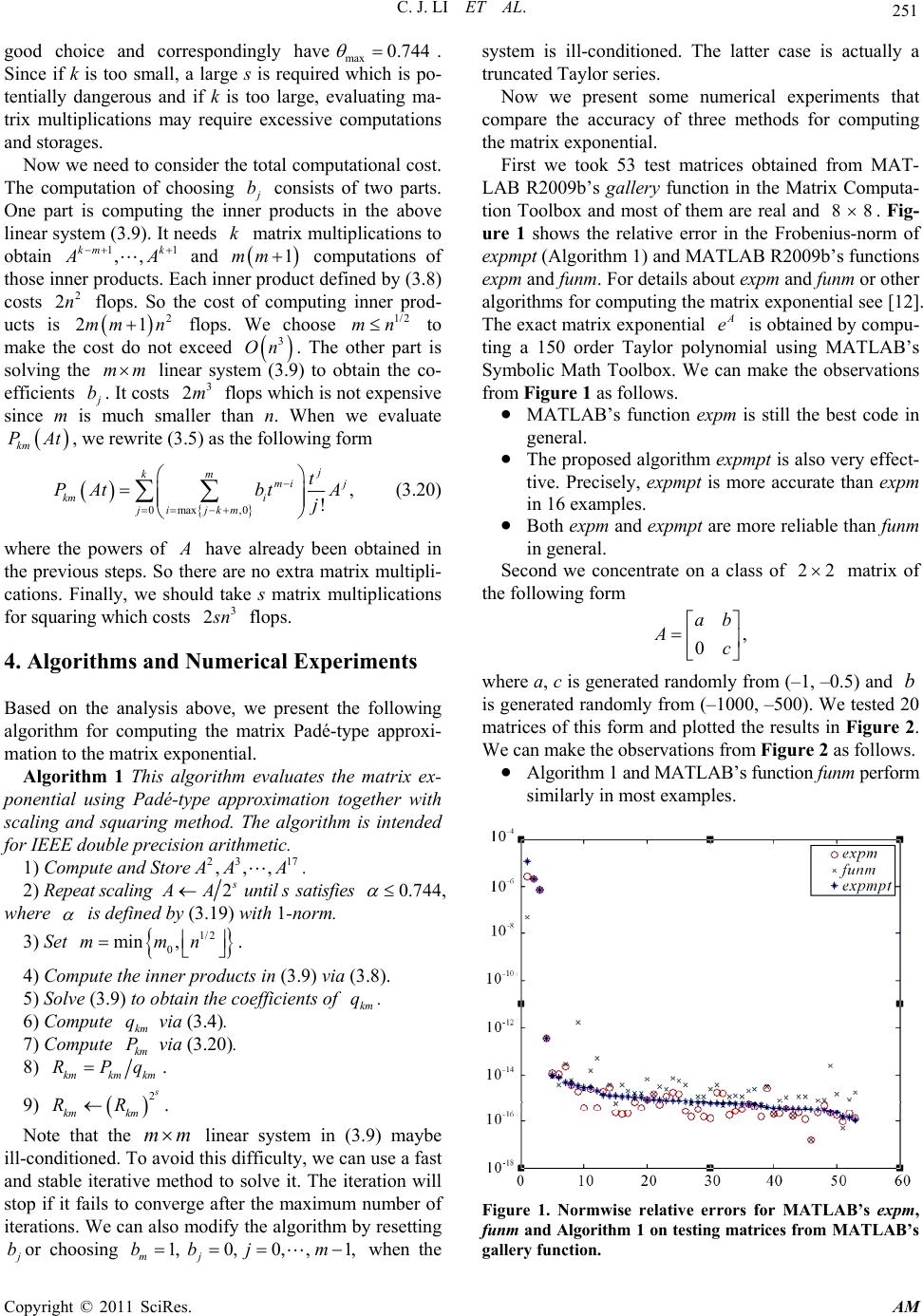

C. J. LI ET AL.
251
good choice and correspondingly havemax0.744


.
Since if k is too small, a large s is required which is po-
tentially dangerous and if k is too large, evaluating ma-
trix multiplications may require excessive computations
and storages.
Now we need to consider the total computational cost.
The computation of choosing
j
b consists of two parts.
One part is computing the inner products in the above
linear system (3.9). It needs k matrix multiplications to
obtain 11
,,
km k
A
A
 
 and

1mm computations of
those inner products. Each inner product defined by (3.8)
costs 2
2n flops. So the cost of computing inner prod-
ucts is

2
21mm n flops. We choose 1/2 mn to
make the cost do not exceed

3
On . The other part is
solving the mm linear system (3.9) to obtain the co-
efficients
j
b. It costs 3 2m flops which is not expensive
since m is much smaller than n. When we evaluate

km
PAt, we rewrite (3.5) as the following form


0max ,0,
!
j
km mi j
km i
ji jkm
t
PAtbt A
j

 




 (3.20)
where the powers of
A
have already been obtained in
the previous steps. So there are no extra matrix multipli-
cations. Finally, we should take s matrix multiplications
for squaring which costs 3 2
s
n flops.
4. Algorithms and Numerical Experiments
Based on the analysis above, we present the following
algorithm for computing the matrix Padé-type approxi-
mation to the matrix exponential.
Algorithm 1 This algorithm evaluates the matrix ex-
ponential using Padé-type approximation together with
scaling and squaring method. The algorithm is intended
for IEEE double precision arithmetic.
1) Compute and Store23 17 ,,,
A
AA.
2) Repeat scaling 2
s
A
A until s satisfies 0.744


,
where

is defined by (3.19) with 1-norm.
3) Set


1/2
0
min ,mmn

 .
4) Compute the inner products in (3.9) via (3.8).
5) Solve (3.9) to obtain the coefficients of km q.
6) Compute km q via (3.4).
7) Compute km P via (3.20).
8) kmkmkm RPq.
9)

2
s
km km
RR.
Note that the mm linear system in (3.9) maybe
ill-conditioned. To avoid this difficulty, we can use a fast
and stable iterative method to solve it. The iteration will
stop if it fails to converge after the maximum number of
iterations. We can also modify the algorithm by resetting
j
bor choosing 1,0,0,,1,
mj
bbj m  when the
system is ill-conditioned. The latter case is actually a
truncated Taylor series.
Now we present some numerical experiments that
compare the accuracy of three methods for computing
the matrix exponential.
First we took 53 test matrices obtained from MAT-
LAB R2009b’s gallery function in the Matrix Computa-
tion Toolbox and most of them are real and 88

. Fig-
ure 1 shows the relative error in the Frobenius-norm of
expmpt (Algorith m 1) and MATLAB R2009 b’s fun ction s
expm and funm. For details about expm and funm or other
algorithms for computing the matrix exponential see [12].
The exact matrix exponential A
e is obtained by compu-
ting a 150 order Taylor polynomial using MATLAB’s
Symbolic Math Toolbox. We can make the observations
from Figure 1 as follows.
 MATLAB’s function expm is still the best code in
general.
 The proposed algorithm expmpt is also very effect-
tive. Precisely, expmpt is more accurate than expm
in 16 examples.
 Both expm and expmpt are more reliable than funm
in general.
Second we concentrate on a class of 22 matrix of
the following form
,
0
ab
Ac







where a, c is generated randomly from (–1, –0. 5) and b
is generated rando mly from (–1000, –500). We tested 20
matrices of this form and plotted the results in Figure 2.
We can make the observations from Figure 2 as follows.
 Algorithm 1 and MATLAB’s function funm perform
similarly in most examples.
Figure 1. Normwise relative errors for MATLAB’s expm,
funm and Algor ithm 1 on testing matrices from MATL AB’s
gallery function.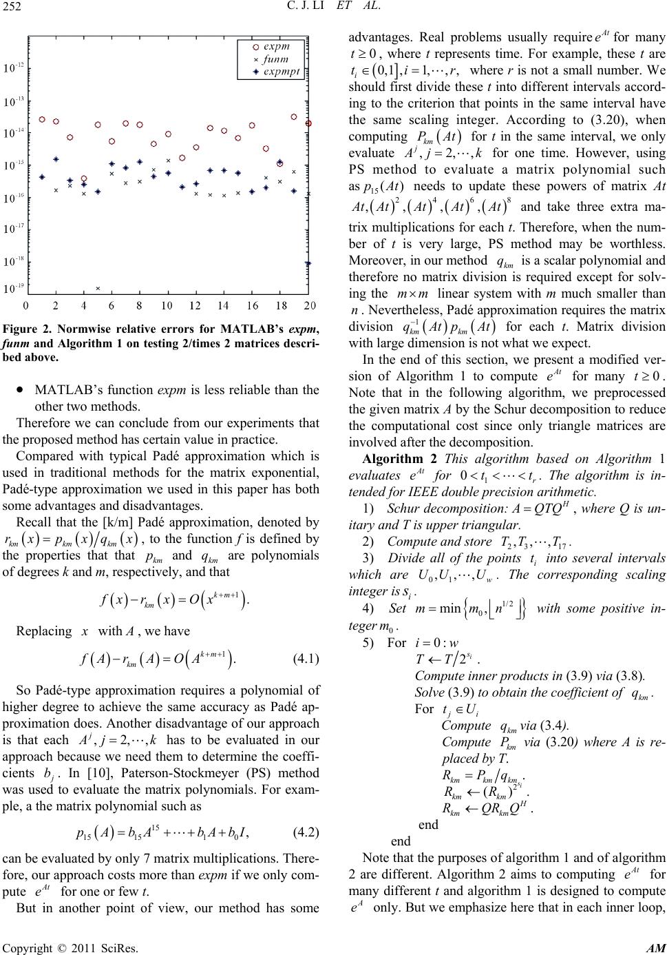

C. J. LI ET AL.
252
Figure 2. Normwise relative errors for MATLAB’s expm,
funm and Algorithm 1 on testing 2/times 2 matrices descri-
bed above.
 MATLAB’s function ex pm is less reliable than the
other two methods.
Therefore we can conclude from our experiments that
the proposed method has certain value in practice.
Compared with typical Padé approximation which is
used in traditional methods for the matrix exponential,
Padé-type approximation we used in this paper has both
some advantages and disadvantages.
Recall that the [k/m] Padé approximation, denoted by
 
kmkm km
rx pxqx, to the function f is defined by
the properties that that km p and km q are polynomials
of degrees k and m, respectively, and that
 

1. km
km
fx r xOx


Replacing
x
with
A
, we have
 

1. km
km
fA rAOA

 (4.1)
So Padé-type approximation requires a polynomial of
higher degree to achieve the same accuracy as Padé ap-
proximation does. Another disadvantage of our approach
is that each ,2,,
j
A
jk has to be evaluated in our
approach because we need them to determine the coeffi-
cients
j
b. In [10], Paterson-Stockmeyer (PS) method
was used to evaluate the matrix polynomials. For exam-
ple, a the matrix polynomial such as

15
151510 ,pAbAbAbI (4.2)
can be evaluated by only 7 matrix multiplications. There-
fore, our approach costs more than expm if we only com-
pute At e for one or few t.
But in another point of view, our method has some
advantages. Real problems usually requireAt
efor many
0t, where t represents time. For example, these t are


0,1 ,1,,,
i
tir where r is not a small number. We
should first divide these t into different intervals accord-
ing to the criterion that points in the same interval have
the same scaling integer. According to (3.20), when
computing


km
PAt for t in the same interval, we only
evaluate ,2,,
j
A
jk for one time. However, using
PS method to evaluate a matrix polynomial such
as 15 ()pAt needs to update these powers of matrix At

2468
,,,,
A
tAtAtAtAt and take three extra ma-
trix multiplications for each t. Therefore, when the num-
ber of t is very large, PS method may be worthless.
Moreover, in our method km q is a scalar polynomial and
therefore no matrix division is required except for solv-
ing the mm

linear system with m much smaller than
n. Nevertheless, Padé approximation requires the matrix
division




1
km km
qAtpAt
 for each t. Matrix division
with large dimension is not what we expect.
In the end of this section, we present a modified ver-
sion of Algorithm 1 to compute At e for many 0t.
Note that in the following algorithm, we preprocessed
the given matrix A by the Schur decomposition to reduce
the computational cost since only triangle matrices are
involved after the decomposition.
Algorithm 2 This algorithm based on Algorithm 1
evaluates At
e for 1 0r tt

. The algorithm is in-
tended for IEEE double precision arithmetic.
1) Schur decomposition:
H
A
QTQ, where Q is un-
itary and T is upper triangular.
2) Compute and store 23 17 ,,,TT T.
3) Divide all of the points i t into several intervals
which are 01
,,,
w
UU U. The corresponding scaling
integer isi
s
.
4) Set


1/2
0
min ,mmn




 with some positive in-
teger 0
m.
5) For 0:iw

2i
s
TT.
Compute inner products in (3.9) via (3.8).
Solve (3.9) to obtain the coefficient of km
q.
For
j
i
tU

Compute km qvia (3.4).
Compute km P via (3.20) where A is re-
placed by T.
kmkmkm
RPq

.
2
()
s
i
km km
RR.
H
km km
RQRQ.
end
end
Note that the purposes of algorithm 1 and of algorithm
2 are different. Algorithm 2 aims to computing At e for
many different t and algorithm 1 is designed to compute
A
e only. But we emphasize here that in each inner loop,

C. J. LI ET AL.
253
algorithm uses the same approach as algorithm 1 to com-
pute eachAt e. In addition, only Schur decomposition is
added at the beginning of the algorithm to reduce the
computational cost when the number t is very much.
Therefore, we do not present any numerical results of al-
gorithm 2.
5. Conclusions
In this paper, we develop a new approach based on ma-
trix Padé-type approximation mixed with the scaling and
squaring method to compute the matrix exponential in-
stead of typical Padé approximation. Two numerical al-
gorithms for computing A
e and forAt ewith many
0t respectively are proposed. Our approach is estab-
lished closely relative to the backward error analysis and
computational considerations. Numerical results com-
paring the proposed algorithm with existing functions
expm and funm in MATLAB have shown the proposed
algorithm is effective and reliable for computing the ma-
trix exponential. Compared with typical Padé approxi-
mation, the most significant advantages of matrix Padé-
type approximation lie in two aspects. One is the con-
venience for computing At
e for a large amount of t. The
other is its avoiding nn matrix divisions, where n is
the size of the given matrix A.
6. Acknowledgements
The authors gratefully acknowledge the fund support
from Applied Mathematics.
7. References
[1] C. B. Moler and C. F. Van Loan, “Nineteen Dubious
Ways to Compute the Exponential of a Matrix,” SIAM
Review, Vol. 20, No. 4, 1978, pp. 801-836.
doi:10.1137/1020098
[2] C. B. Moler and C. F. Van Loan, “Nineteen Dubious
Ways to Compute the Exponential of a Matrix, Twenty-
Five Years Later,” SIAM Review, Vol. 45, No. 1, 2003,
pp. 3-49. doi:10.1137/S00361445024180
[3] N. J. Higham, “The Scaling and Squaring Method for the
Matrix Exponential Revisited,” SIAM Journal on Matrix
Analysis and Application, Vol. 26, No. 4, 2005, pp. 1179-
1193. doi:10.1137/04061101X
[4] N. J. Higham, “The Scaling and Squaring Method for the
Matrix Exponential Revisited,” SIAM Review, Vol. 51,
No. 4, 2009, pp. 747-764. doi:10.1137/090768539
[5] C. Gu, “Matrix Padé-Type Approximant and Directional
Matrix Padé Approximant in the Inner Product Space,”
Journal of Computational and Applied Mathematics, Vol.
164-165, No. 1, 2004, pp. 365-385.
doi:10.1016/S0377-0427(03)00487-4
[6] C. Brezinski, “Rational Approximation to Formal Power
Series,” Journal of Approximation Theory, Vol. 25, No. 4,
1979, pp. 295-317. doi:10.1016/0021-9045(79)90019-4
[7] C. Brezinski, “Padé-Type Approximation and General
Orthogonal Polynomials,” Birkh Äauser-Verlag, Basel,
1980.
[8] A. Draux, “Approximants de Type Padé et de Table,”
Little: Publication A, University of Lille, Lille, No. 96,
1983.
[9] C. Gu, “Generalized Inverse Matrix Padé Approximation
on the Basis of Scalar Products,” Linear Algebra and Its
Applications, Vol. 322, No. 1-3, 2001, pp. 141-167.
doi:10.1016/S0024-3795(00)00230-5
[10] C. Gu, “A Practical Two-Dimensional Thiele-Type Ma-
trix Padé Approximation,” IEEE Transactions on Auto-
matic Control, Vol. 48, No. 12, 2003, pp. 2259-2263.
doi:10.1109/TAC.2003.820163
[11] N. J. Higham, “Functions of Matrices: Theory and Com-
putation,” SIAM Publisher, Philadelphia, 2008.
doi:10.1137/1.9780898717778
[12] A. Sidi, “Rational Approximations from Power Series of
Vector-Valued Meromorphic Functions,” Journal of Ap-
proximation Theory, Vol. 77, No. 1, 1994, pp. 89-111.
doi:10.1006/jath.1994.1036
[13] R. Mathias, “Approximation of Matrix-Valued Functions,”
SIAM Journal on Matrix Analysis and Application, Vol.
14, No. 4, 1993, pp. 1061-1063. doi:10.1137/0614070
[14] J. D. Lawson, “Generalized Runge-Kutta Processes for
Stable Systems with Large Lipschitz Constants,” SIAM
Journal on Numerical Analysis, Vol. 4, No. 3, 1967, pp.
372-380. doi:10.1137/0704033
[15] A. H. Al-Mohy and N. J. Higham, “A New Scaling and
Squaring Algorithm for the Matrix,” SIAM Journal on
Matrix Analysis and Application, Vol. 31, No. 3, 2009, pp.
970-989. doi:10.1137/09074721X