Applied Mathematics, 2011, 2, 236-240
doi:10.4236/am.2011.22026 Published Online February 2011 (http://www.SciRP.org/journal/am)
Improving AOR Method for a Class of Two-by-Two
Linear Systems
Cuixia Li1, Shiliang Wu2
1College of Mathematics, Chengdu University of Infromation Technology, Chengdu, China
2School of Mathema tics and Statistics, Anyang Normal University, Anyang, China
Received October 18, 2010; revised December 10, 2010; accepted December 15, 2010
Abstract
In this paper, the preconditioned accelerated overrelaxation (AOR) method for solving a class of two-by-two
linear systems is presented. A new preconditioner is proposed according to the idea of [1] by Wu and Huang.
The spectral radii of the iteration matrix of the preconditioned and the original methods are compared. The
comparison results show that the convergence rate of the preconditioned AOR methods is indeed better than
that of the original AOR methods, whenever the original AOR methods are convergent under certain condi-
tions. Finally, a numerical example is presented to confirm our results.
Keywords: Preconditioner, AOR Method, Convergence, Comparison
1. Introduction
Sometimes we have to solve the following linear systems
,
H
xf (1.1)
where
1
2
,
IB D
HCIB





is non-singular with








12
,,
,.
ij ij
ppnp np
ij ij
nppp np
Bb Bb
Cc Dd

 


Systems such as (1.1) are important and appear in
many different applications of scientific computing. For
example, (1.1) are usually faced when the following gen-
eralized linear-squares problem is considered

1
min ,
n
T
x
A
xbWAxb



where Wis the variance-covariance matrix. One can see
[2-5] for details.
As is known, the linear systems (1.1) can be solved by
direct methods or iterative methods. Direct methods are
widely employed when the order of the coefficient ma-
trix
H
is not too large, and are often regarded as robust
methods. The memory and the computational require-
ments for solving the large linear systems may seriously
challenge the most efficient direct methods available to-
day. The alternative is to use iterative methods establi-
shed for solving the large linear systems. Naturally, it is
necessary that we make the use of iterative methods in-
stead of direct methods to solve the large sparse linear
systems. Meanwhile, iterative methods are easier to im-
plement efficiently on high performance computers than
direct methods.
As is known, there exist three well-known classical it-
erative methods, i.e., Jacobi, Gauss-Seidel and succes-
sive overrelaxation (SSOR) method, which were fully
covered in the excellent books by Varge [6] and Young
[7]. To make the convergence rate of SSOR method bet-
ter, accelerated overrelaxation (AOR) method was pro-
posed in [8] by Hadjidimos.
To solve the linear systems (1.1) with the AOR itera-
tive method, based on the structure of the matrix
H
, the
matrix
H
is split as follows
1
2
00 .
0 0
BD
HI B
C




 
 

 
(1.2)
The AOR iterative method for solving (1.1) is estab-
lished as follows
  1
,,0,1,
ii
wr
xTxwgi
 (1.3)
where 0w

, ,wr T is iteration matrix and is of the fol-
lowing form

C. X. LI ET AL.
237


 
1
1
,
2
1
12
000
10
0
1
11
wr
BD
I
TwIw
B
rC IC
w IwBwD
wrC wrCBwIwBwrCD




 



  



  

 

 

and
0. I
g
f
rC I




Obviously, if wr , then the AOR method reduces to
the SOR method.
The spectral radii of the iteration matrix is decisive for
the convergence and stability of the method, and the
smaller it is, the faster the method converges when the
spectral radii is smaller than 1. To accelerate the conver-
gence rate of the iterative method solving the linear sys-
tems (1.1), preconditioned methods are often used. That
is,
,PHx Pf
where the preconditioner P is a non-singular matrix.
If the matrix PH is expressed as
1
2
,
IB D
PH CIB








then the preconditioned AOR method can be defined by
 

,
1,0,1,
wr
ii
xTxwgwi

 (1.4)
where

 
1
,
12
1
11
wr
w IwBwD
TwrCwrCBwI wBwrCD


 

 

 


and
0. I
g
Pf
rC I






In this paper, according to the idea of [1] by Wu and
Huang, a new preconditioner is proposed to improve the
convergence rate of the AOR method. Be similar to the
work of [1] and [9], we compare the spectral radii of the
iteration matrix of the preconditioned and the original
methods. The comparison results show that the conver-
gence rate of the preconditioned AOR methods is indeed
superior to that of the original AOR methods, whenever
the original AOR methods are convergent (to see the next
section).
For convenience, we shall now briefly explain some of
the terminology and lemmas. Let

nn
ij
Cc

 be an
nn real matrix. By

,diag C we denote thenn

di-
agonal matix coinciding in its diagonal with .
ii
c For

,
ij
A
a

,
nn
ij
Bb  we write
A
Bif ij ij ab
holds for all ,1,2,,.ij n

 Calling
A
is nonnegative
if 0,A


0;,1,2,,,
ij
aij nwe say that 0AB


if and only if
A
B These definitions carry immedi-
ately over to vectors by identifying them with 1n

ma-
trices.




denotes the spectral radius of a matrix.
Lemma 1.1 [6] Let nn
A


 be a nonnegative and
irreducible nn

matrix. Then
1)
A
has a positive real eigenvalue equal to its spec-
tral radius


A
 ;
2) for


,
A
 there corresponds an eigenvector 0x;
3)


A
 is a simple eigenvalue of
A
.
4)


A
 increases when any entry of
A
increases.
Lemma 1.2 [10] Let
A
be a nonnegative matrix.
Then
1) If
x
Ax


for some nonnegative vector ,
x
0x

, then


A
 .
2) If
A
xx


for some positive vector
x
, then


A



. Moreover, if
A
is irreducible and if
0
x
Ax x



 for some nonnegative vector
x
, then
()A




and
x
is a positive vector.
The outline of this paper is as follows. In Section 2,
the spectral radii of the iteration matrix of the original
and the preconditioned methods are compared. In Sec-
tion 3, a numerical example is presented to illustrated our
results.
2. Preconditioned AOR Methods and
Comparisons
Now, let us consider the preconditioned linear systems,
,
H
xf

  (2.1)
where


H
ISH
  and

f
ISf
with
0.
00
S
S








According to [1], here S is taken as as follows
12
23
1,
,1
0 00
00 0
.
000
00 0
pp
p
p
p
b
b
S
b
b















Naturally, we assume that there at least exists a non-
zero number in the elements of S.
By simple computations, we obtain

 
11
2
I
BSIB ISD
HCIB


 











C. X. LI ET AL.
238
with

11
1112 2112 22112 2
2123 312223 32223 3
1112 11211
.
pp
pp
ppp pppp
BSIB
bbbbbbbb
bbbbbbb bb
bbb bbb bb




 










Be similar to (1.2),
H
 can be expressed as

 
11
2
00 .
00
BSIB ISD
HI CB
 
 
 



 

Then the preconditioned AOR method for (2.1) is de-
fined as follows:
 

1
,,00,1,
ii
wr
xTxwgwi

 (2.2)
where



,11
11
2
11
1
wr
TwIwBSIBwrC
wrCBSIBw ISDw I
wBwrC IS D

 






 


and
0. I
g
f
rC I






The following theorem is given by comparing the
spectral radii of the iteration matrix ,wr
T
 and the origi-
nal iteration matrix ,wr
T.
Theorem 2.1 Let the coefficient matrix
H
be irre-
ducible, 10B with

10diag B, 20B, 0C

,
0D, 01w and 01r. Then
1)
 
,,
,
wr wr
TT  
 if


,1; wr
T  
2)


,,
,
wr wr
TT  
 if


,1. wr
T  
Proof. By simple computations, we obtain

 
1
,
2
1
1
11
00
wr
w IwBwD
TwrCwI wB
wr CB CD
 




 


(2.3)
Clearly, if the matrix
H
satisfies 10B, 20B,
0C and 0D with 01w and 01r, then
,
1
00
0 and0.
wr
T
CB CD





Since the matrix
H
is irreducible, by observing the
structure of (2.3), it is not difficult to get that the matrix
,wr
T is irreducible. Similarly, the matrix ,wr T
 is non-
negative and irreducible with

10diag B.
By Lemma 1.1, there is a positive vector
x
such that
,, wr
Tx x


Where


,. wr
T  Obviously, 1

 is impossible,
otherwise the matrix
H
becomes singular. So we will
mainly discuss two cases: 1

 and 1

.
Case 1: 1


. Since ,,, ,
wrwr wr
Tx xTxTx  
 we
get






1
,,
1
1
,
0
000
0
0
0
1.
0
wr wr
wr
wS IBwSD
TxTx x
wrCS IBwrCSD
SwI BwD
x
rCS
STIx
rCS
Sx
rCS

 




  
















Since 0S and 0S

, then we get
00
0and 0.
00
SS
xx
rCS rCS
 
 
 

 
If 1


, then ,, 0
wr wr
TxTx


 but not equal to zero
vector. By Lemma 1.2, we get


,,wr wr
TT  
. That
is, 1) holds.
Similarly, 2) holds with 1,

 which completes the
proof. □
It is well known that when wr , AOR iteration is
reduced to SOR iteration. The following corollary is eas-
ily obtained.
Corollary 2.1 Let the coefficient matrix
H
be irre-
ducible, 10B with

10diag B, 20B, 0C

,
0D

and 01w

. Then
1)




,
ww
TT  
 if

1;
w
T  
2)




,
ww
TT  
 if

1.
w
T  
Next, we consider the following preconditioners. Let
the matrix S
 in (2.1) be defined by
00
.
0
SS








There exist the following three forms for S, that is,
1) If npp

, then

11
22
,1 ,
0000
0000
.
000
npnpnp np p
c
c
S
cc
















2) If npp

, then

11
22
,1 ,
00
00
.
0
npnpnp np p
c
c
S
cc

















C. X. LI ET AL.
239
3) If np p, then

11
22
,1 ,
00
00
.
0
00 0
ppp
npp
c
c
Scc




















Naturally, we assume that there at least exists a non-
zero number in the elements of S. For the sake of sim-
plicity, we assume that ,npp
H
 can be expressed
as

1
12
IB D
HSI BC I BSD



 


with

1
11 111211 12111 1
2122 2122 22222 2
,1 ,2,
pp
pp
np npnpp
SI BC
cbc cbccb
ccbcbc cb
dd d
 














where
,1,1 11,,1
,2,2 ,112 ,,2
,,,11,,
,
,
.
np npnpnpnp
npnpnpnpnpnp
n ppn ppn ppn pnp n pp
dcbcb
dccbcb
dccbcb
 



 

 

The matrix
H
 is split as follows

1
12
00 .
00
BD
HI SI BCBSD
 

 






Then the preconditioned AOR method for (2.1) is of
the following form:
 

1
,,00,1,
ii
wr
xTxwgw i

where

,1, wr
TwIwJwrK 

1
12
,
BD
JSI BC BSD





   
111
00
,KSI BCI BSIBCD


 

and


1
0. I
g
f
rSI BCI




Similarly, the following theorem and corollary are
given by comparing the spectral radii of the iteration ma-
trix ,wr
T and the original iteration matrix ,wr T.
Theorem 2.2 Let the coefficient matrix
H
be irre-
ducible, 10Bwith


10,diag B20,B0,C

0D

,
01w

 and 01r

. Then
1)




,,
,
wr wr
TT   if

,1; wr
T  
2)




,,
,
wr wr
TT   if

,1. wr
T  
Corollary 2.2 Let the coefficient matrix
H
be irre-
ducible, 10Bwith


10,diag B20,B0,C

0D

,
and 01w

. Then
1)




,
ww
TT   if

1;
w
T  
2)




,
ww
TT   if

1.
w
T  
3. A Numerical Example
Now let us consider the following example to illustrate
the results.
Example 3.1
1
2
,
IB D
HCIB









where






12
12
,,
ij ij
ppnp np
Bb Bb





,
ij np p
Cc

 and


ij
p
np
Dd 
with



1
1
1,1,2,,,
50
11
,,
40 40
1, ,1,2, ,
ii
ij
bi p
bij
ji
ipjp









111
,,
40 401
2, ,,1,2, ,1
ij
bij
ij i
ipj p
 
 






2
2
1,1,2,,,
40
11
,,
40 40
1, ,1,2,,
ii
ij
bi np
bij
pj pi
inpjnp
 
 


 





211
,,
40 401
2, ,,2,,1
ij
bij
ij pi
inpjnp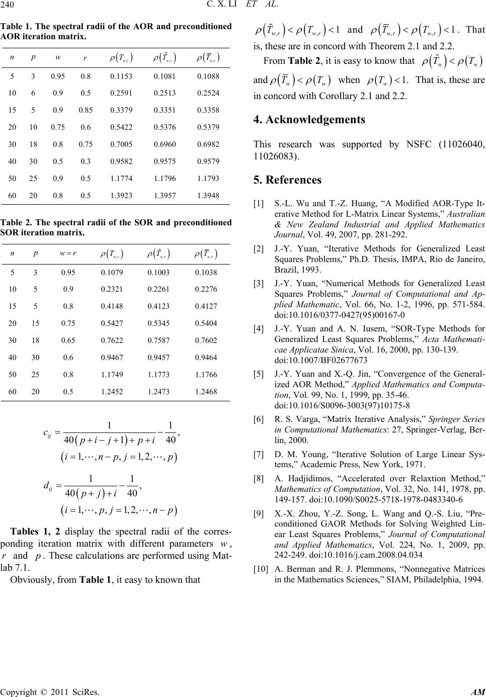
 
 

  

C. X. LI ET AL.
240
Table 1. The spectral radii of the AOR and preconditioned
AOR iteration matrix.
n
p
w r

,wr
T 

,wr
T 



,wr
T 
5 3 0.95 0.8 0.1153 0.1081 0.1088
10 6 0.9 0.5 0.2591 0.2513 0.2524
15 5 0.9 0.85 0.3379 0.3351 0.3358
20 10 0.75 0.6 0.5422 0.5376 0.5379
30 18 0.8 0.75 0.7005 0.6960 0.6982
40 30 0.5 0.3 0.9582 0.9575 0.9579
50 25 0.9 0.5 1.1774 1.1796 1.1793
60 20 0.8 0.5 1.3923 1.3957 1.3948
Table 2. The spectral radii of the SOR and preconditioned
SOR iteration matrix.
n
p
wr

,wr
T 

,wr
T 



,wr
T 
5 3 0.95 0.1079 0.1003 0.1038
10 5 0.9 0.2321 0.2261 0.2276
15 5 0.8 0.4148 0.4123 0.4127
20 15 0.75 0.5427 0.5345 0.5404
30 18 0.65 0.7622 0.7587 0.7602
40 30 0.6 0.9467 0.9457 0.9464
50 25 0.8 1.1749 1.1773 1.1766
60 20 0.5 1.2452 1.2473 1.2468


11
,
401 40
1, ,,1,2,,
ij
cpi jpi
inpj p

 



11
,
40 40
1, ,,1,2, ,
ij
dpj i
ipj np



Tables 1, 2 display the spectral radii of the corres-
ponding iteration matrix with different parameters w,
r and p. These calculations are performed using Mat-
lab 7.1.
Obviously, from Table 1, it easy to known that




,,
1
wr wr
TT 


 and


,,
1
wr wr
TT  . That
is, these are in concord with Theorem 2.1 and 2.2.
From Table 2, it is easy to know that



ww
TT  

and




ww
TT   when

1.
w
T   That is, these are
in concord with Corollary 2.1 and 2.2.
4. Acknowledgements
This research was supported by NSFC (11026040,
11026083).
5. References
[1] S.-L. Wu and T.-Z. Huang, “A Modified AOR-Type It-
erative Method for L-Matrix Linear Systems,” Australian
& New Zealand Industrial and Applied Mathematics
Journal, Vol. 49, 2007, pp. 281-292.
[2] J.-Y. Yuan, “Iterative Methods for Generalized Least
Squares Problems,” Ph.D. Thesis, IMPA, Rio de Janeiro,
Brazil, 1993.
[3] J.-Y. Yuan, “Numerical Methods for Generalized Least
Squares Problems,” Journal of Computational and Ap-
plied Mathematic, Vol. 66, No. 1-2, 1996, pp. 571-584.
doi:10.1016/0377-0427(95)00167-0
[4] J.-Y. Yuan and A. N. Iusem, “SOR-Type Methods for
Generalized Least Squares Problems,” Acta Mathemati-
cae Applicatae Sinica, Vol. 16, 2000, pp. 130-139.
doi:10.1007/BF02677673
[5] J.-Y. Yuan and X.-Q. Jin, “Convergence of the General-
ized AOR Method,” Applied Mathematics and Computa-
tion, Vol. 99, No. 1, 1999, pp. 35-46.
doi:10.1016/S0096-3003(97)10175-8
[6] R. S. Varga, “Matrix Iterative Analysis,” Springer Series
in Computational Mathematics: 27, Springer-Verlag, Ber-
lin, 2000.
[7] D. M. Young, “Iterative Solution of Large Linear Sys-
tems,” Academic Press, New York, 1971.
[8] A. Hadjidimos, “Accelerated over Relaxtion Method,”
Mathematics of Computation, Vol. 32, No. 141, 1978, pp.
149-157. doi:10.1090/S0025-5718-1978-0483340-6
[9] X.-X. Zhou, Y.-Z. Song, L. Wang and Q.-S. Liu, “Pre-
conditioned GAOR Methods for Solving Weighted Lin-
ear Least Squares Problems,” Journal of Computational
and Applied Mathematics, Vol. 224, No. 1, 2009, pp.
242-249. doi:10.1016/j.cam.2008.04.034
[10] A. Berman and R. J. Plemmons, “Nonnegative Matrices
in the Mathematics Sciences,” SIAM, Philadelphia, 1994.