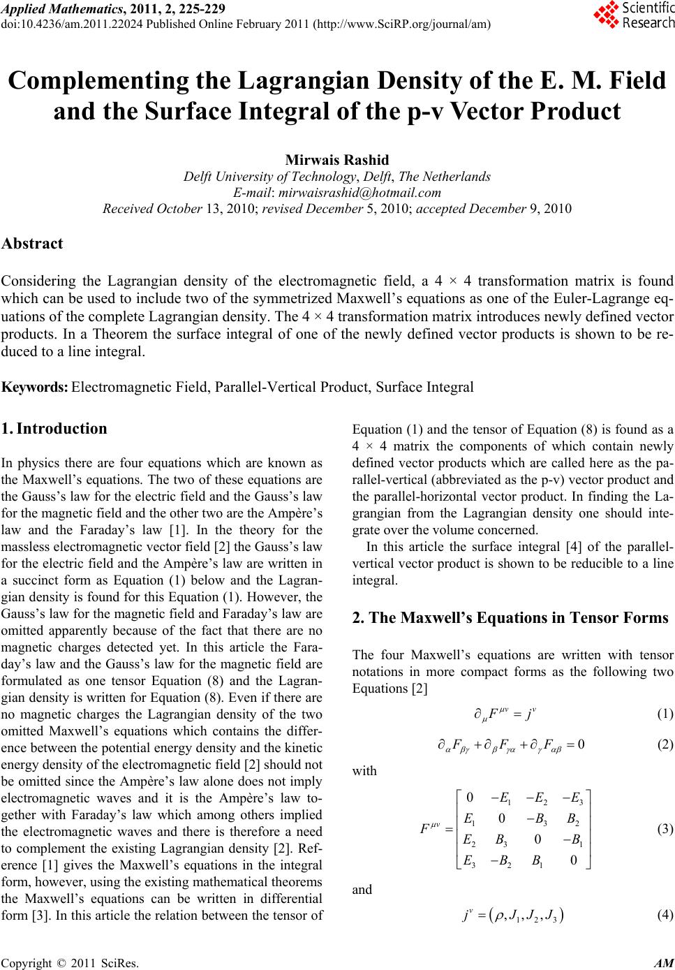Applied Mathematics, 2011, 2, 225-229
doi:10.4236/am.2011.22024 Published Online February 2011 (http://www.SciRP.org/journal/am)
Complementing t he La gr angian Density o f t he E . M . Fi eld
and the Surface Integral of the p-v Vector Produc t
Mirwais Rashid
Delft University of Technology, Delft, The Netherlands
Received October 13, 2010; revised December 5, 2010; accepted December 9, 2010
Abstract
Considering the Lagrangian density of the electromagnetic field, a 4 × 4 transformation matrix is found
which can be used to include two of the symmetrized Maxwell’s equations as one of the Euler-Lagrange eq-
uations of the complete Lagrangian density. The 4 × 4 transformation matrix introduces newly defined vector
products. In a Theorem the surface integral of one of the newly defined vector products is shown to be re-
duced to a line integral.
Keywords: Electromagnetic Field, Parallel-Vertical Product, Surface Integral
1. Introduction
In physics there are four equations which are known as
the Maxwell’s equations. The two of these equations are
the Gauss’s law for the electric field and the Gauss’s law
for the magnetic field and the other two are the Ampère’s
law and the Faraday’s law [1]. In the theory for the
massless electromagnetic vector field [2] the Gauss’s law
for the electric field and the Ampère’s law are written in
a succinct form as Equation (1) below and the Lagran-
gian density is found for this Equation (1). However, the
Gauss’s law for the magnetic field and Faraday’s law are
omitted apparently because of the fact that there are no
magnetic charges detected yet. In this article the Fara-
day’s law and the Gauss’s law for the magnetic field are
formulated as one tensor Equation (8) and the Lagran-
gian density is written for Equatio n (8). Even if there are
no magnetic charges the Lagrangian density of the two
omitted Maxwell’s equations which contains the differ-
ence between the potential energy density and the kinetic
energy density of the electromagnetic field [2] should not
be omitted since the Ampère’s law alone does not imply
electromagnetic waves and it is the Ampère’s law to-
gether with Faraday’s law which among others implied
the electromagnetic waves and there is therefore a need
to complement the existing Lagrangian density [2]. Ref-
erence [1] gives the Maxwell’s equations in the integral
form, however, using the existing mathematical theorems
the Maxwell’s equations can be written in differential
form [3]. In this article the relation between the tensor of
Equation (1) an d the tensor of Equation (8) is found as a
4 × 4 matrix the components of which contain newly
defined vector products which are called here as the pa-
rallel-vertical (abbreviated as the p-v) vector product and
the parallel-horizontal vector product. In finding the La-
grangian from the Lagrangian density one should inte-
grate over the vol ume concerned.
In this article the surface integral [4] of the parallel-
vertical vector product is shown to be reducible to a line
integral.
2. The Maxwell’s Equations in Tensor Forms
The four Maxwell’s equations are written with tensor
notations in more compact forms as the following two
Equations [2]
vv
F
j



 (1)
0FFF


 (2)
with
123
132
23 1
321
0
0
0
0
v
EEE
EBB
FEB B
EBB


















(3)
and


123
,,,
v
jJJJ   (4)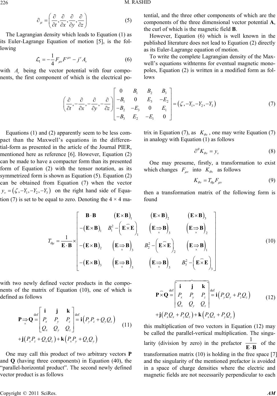

M. RASHID
226
,,,
txyz

 


  

(5)
The Lagrangian density which leads to Equation (1) as
its Euler-Lagrange Equation of motion [5], is the fol-
lowing
11
4
vv
vv
F
FjA


  (6)
with v
A
being the vector potential with four compo-
nents, the first component of which is the electrical po-
tential, and the three other components of which are the
components of the three dimensional vector potential A,
the curl of which is the magnetic field B.
However, Equation (6) which is well known in the
published literature does not lead to Equation (2) d irectly
as its Euler-Lagrange equation of motion.
To write the complete Lagran gian density of the Max-
well’s equations withterms for eventual magnetic mono-
poles, Equation (2) is written in a modified form as fol-
lows

123
132
123
231
32 1
0
0
,,, ,,,
0
0
BBB
BEE
YYY
BEE
txyz
BE E




  

 


  




(7)
Equations (1) and (2) apparently seem to be less com-
pact than the Maxwell’s equations in the differen-
tial-form as presented in the article of the Journal PIER,
mentioned here as reference [6]. However, Equation (2)
can be made to have a compacter form than its presented
form of Equation (2) with the tensor notation, as its
symmetrized form is shown as Equation (5). Equation (2)
can be obtained from Equation (7) when the vector

123
,,,
v
y
YYY   on the right hand side of Equa-
tion (7) is set to be equal to zero. Denoting the 4 × 4 ma-
trix in Equation (7), as v
K

, one may write Equation (7)
in analogy with Equation (1) as follo ws
vv
K
y



 (8)
One may presume, firstly, a transformation to exist
which changes v
F

into v
K

as follows
vv
K
TF

 

(9)
then a transformation matrix of the following form is
found












123
2
1
132
1
2
2
231
2
2
3
333 3
1
B
TB
B




 



 




 

  






 


BB EBEBEB
EBEEE BE B
EB EBEEEB EB
EBE BE BEE



(10)
with two newly defined vector products in the compo-
nents of the matrix of Equation (10), one of which is
defined as follows



def def
x
yz yzyz
xyz
xzx zxyxy
PPP PPQQ
QQQ
PP QQPPQQ



 



 
ijk
PQ i
jk
(11)
One may call this product of two arbitrary vectors P
and Q (having three components) in Equation (40), the
“parallel-horizontal product”. The second newly defined
vector product is as follows

 
def def
x
yz yyzz
xyz
xx zzxxyy
P
PP PQPQ
QQQ
PQ PQPQ PQ


 



 
ijk
PQ i
jk


  
(12)
this multiplication of two vectors in Equation (12) may
be called the parallel-vertical multiplication. The singu-
larity (division by zero) in the prefactor 1

EB of the
transformation matrix (10) is holding in the free space [7]
and the singularity of th e mentioned prefactor is avoided
in a space of charge densities where the electric and
magnetic fields are not necessarily perpendicular to each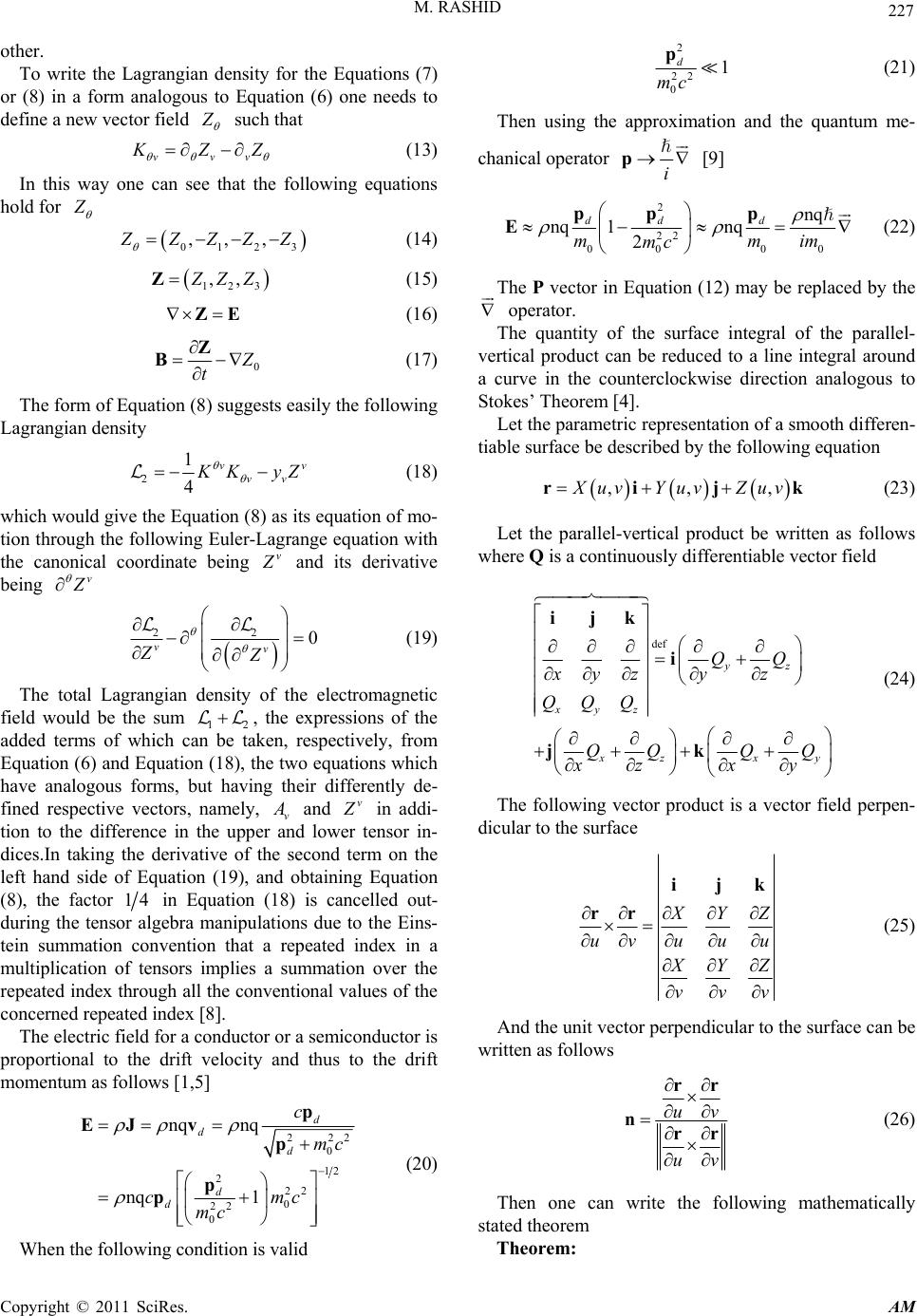

M. RASHID
227
other.
To write the Lagrangian density for the Equations (7)
or (8) in a form analogous to Equation (6) one needs to
define a new vector field
Z

such that
vvv
K
ZZ


 (13)
In this way one can see that the following equations
hold for
Z


0123
,,,
Z
ZZZZ

 (14)

123
,,
Z
ZZZ (15)
 ZE (16)
0
Z
t



Z
B (17)
The form of Equation (8) suggests easily the following
Lagrangian density
21
4
vv
vv
K
KyZ


  (18)
which would give the Equation (8) as its equation of mo-
tion through the following Euler-Lagrange equation with
the canonical coordinate being v
Z
and its derivative
being v
Z



22
0
vv
ZZ





 




(19)
The total Lagrangian density of the electromagnetic
field would be the sum 12 , the expressions of the
added terms of which can be taken, respectively, from
Equation (6) and Equation (18), the two equations which
have analogous forms, but having their differently de-
fined respective vectors, namely, v
A
and v
Z
in addi-
tion to the difference in the upper and lower tensor in-
dices.In taking the derivative of the second term on the
left hand side of Equation (19), and obtaining Equation
(8), the factor 14 in Equation (18) is cancelled out-
during the tensor algebra manipulations due to the Eins-
tein summation convention that a repeated index in a
multiplication of tensors implies a summation over the
repeated in dex through all the conventional v alues of the
concerned repeated index [8].
The electric field for a conductor or a semiconductor is
proportional to the drift velocity and thus to the drift
momentum as follows [1,5]
222
0
12
222
0
22
0
nq nq
nq 1
d
d
d
d
d
c
mc
cmc
mc
 


 



 



p
EJ vp
p
p
(20)
When the following condition is valid
2
22
0
1
d
mc
p (21)
Then using the approximation and the quantum me-
chanical operator i  p


 [9]
2
22
000 0
nq
nq 1nq
2
dd d
mmim mc







pp p
E


 (22)
The P vector in Equation (12) may be replaced by the


 operator.
The quantity of the surface integral of the parallel-
vertical product can be reduced to a line integral around
a curve in the counterclockwise direction analogous to
Stokes’ Theorem [4].
Let the parametric representation of a smooth differen-
tiable surface be described by the following equation




,,,
X
uvYuvZ uvrijk (23)
Let the parallel-vertical product be written as follows
where Q is a continuously differentiable vector field
def
yz
xyz
x
zxy
QQ
xyzy z
QQQ
QQ QQ
xz xy


  




 




  

 





ijk
i
jk

  
(24)
The following vector product is a vector field perpen-
dicular to the surface
X
YZ
uvuu u
X
YZ
vvv









ijk
rr (25)
And the unit vector perpendicular to the surface can be
written as follows
uv
uv











rr
nrr (26)
Then one can write the following mathematically
stated theorem
Theorem: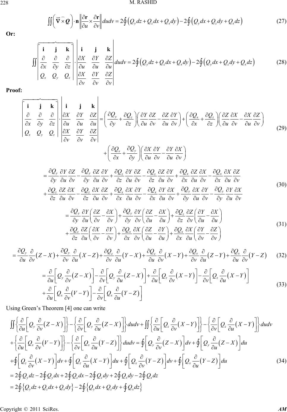

M. RASHID
228

22
yzx yzx
dudvQdzQ dxQ dyQdxQ dyQ dz
uv


  



 
rr
n


︷Q (27)
Or:

22
yzx yzx
xyz
XYZ
dudvQdzQ dxQ dyQdxQ dyQ dz
xyzu uu
XYZ
QQQ vvv


 



  





 
ijki jk


(28)
Proof:
yx
zz
xyz
y
x
QQ
QQ
X
YZYZ ZYZXXZ
x
yzuuuyzuvuvxzuv uv
XYZ
QQQ vvv
Q
QXY YX
xyuvuv

 
 
  
  



  

  
  








 







ijkijk

(29)
yy xx
zz
yy
xx zz
QQ QQ
QQ YZ ZY YZZY ZXXZ
yuvyuv zuvzuv xuvxuv
QQ
QQ
QQ
Z
XXZXYYXXYYX
zuvzuv xuvxuvyuv yuv
 
  

   


    

    
(30)
yyz
xx z
QQQ
YZ XYZ XZY X
yu vvyv uuzv uu
QQ Q
Z
XY XZY XYZ
zu vvxv uuxuvv

   
 

 

  
 
   
  

  

 
  
(31)
  
yy xx
zz
QQ QQ
QQ
Z
XXZYXXYZYYZ
uvvuvuuvvu uv
 


 
 (32)
  
 
yy zz
xx
QZX QZXQXY QXY
uvvuuv vu
QVY QYZ
uv vu






 



 

(33)
Using Green’s Theorem [4] one can write
  
   
yy zz
xx yy
z
QZXQZXdudvQX YQX Ydudv
uvvuuvvu
QVYQYZdudvQZ XdvQZ Xdu
uv vuvu
Q

 


 
 
 


 


 
 
 


 

   
 
222222
22
zxx
yyzzxx
yzxyz x
XYdvQXYduQ YZdv QYZdu
vuvu
QdzQdxQ dxQ dyQ dyQ dz
QdzQdxQ dyQdxQ dyQ dz


 

 






 


(34)

M. RASHID
229
Which proves the Theorem.
3. Conclusions
The Lagrangian density of the electromagnetic field is
complemented here by including a Lagrangian density
for two of the symmetrized Maxwell’s equations.In this
procedure a transformation matrix is found which is in-
cluding in its components two new definitions of vector
products which are called here the “parallel-horizontal”
and “parallel-vertical” vector products. The Theorem of
the surface integral of the parallel-vertical vector product
is shown to be reduced to a line integral.
4. References
[1] D. H. Young and R. A. Freedman, “University Physics,”
9th Edition, Addison-Wesley Publishing Company, Inc.,
USA, 1996.
[2] W. E. Burcham and M. Jobes, “Nuclear and Particle Psy-
sics,” Addison Wesley Longman Limited, Singapore,
1997.
[3] E. M. Purcell, “Electricity and Magnetism,” Berkeley
Physics Course, 2nd Edition, McGraw-Hill, Inc., USA,
Vo l . 2, 1985.
[4] T. M. Apostol, “Calculus,” 2nd Edition, John Wiley &
Sons, Singapore, Vol. 2, 1969.
[5] J. B. Marion and S. T. Thornton, “Classical Dynamics of
Particles and Systems,” 4th Edition, Harcourt Brace &
Co., USA, 1995.
[6] I. V. Lindell, “Electromagnetic Wave Equation in Diffe-
rential-Form Representation,” Progress in Electromag-
netics Research, Vol. 54, 2005, pp. 321-333.
doi:10.2528/PIER05021002
[7] G. R. Fowles, “Introduction to Modern Optics,” 2nd Edi-
tion, Dover Publications, Inc., New York, 1989.
[8] R. D’Inverno, “Introducing Einstein’s Relativity,” Cla-
rendon Press, Oxford, 1995.
[9] S. Gasiorowicz, “Quantum Physics,” 2nd Edition, John
Wiley & Sons, Inc., USA, 1996.