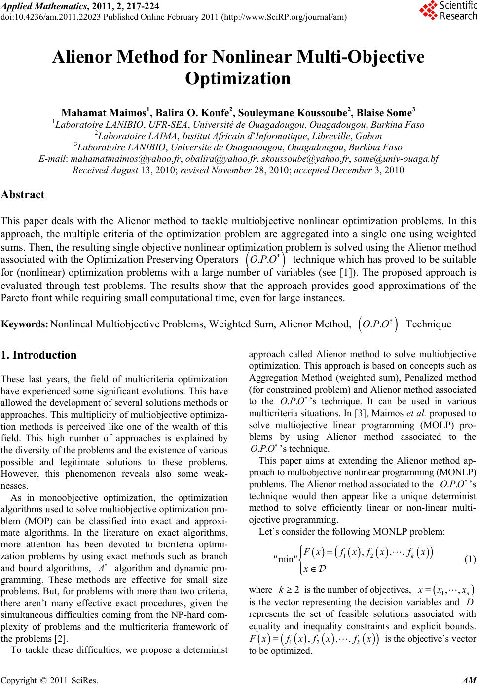Applied Mathematics, 2011, 2, 217-224
doi:10.4236/am.2011.22023 Published Online February 2011 (http://www.SciRP.org/journal/am)
Alienor Method for Nonlinear Multi-Objective
Optimization
Mahamat Maimos1, Balira O. Konfe2, Souleymane Koussoube2, Blaise Some3
1Laboratoire LANIBIO, UFR-SEA, Université de Ouagadougou, Ouagadougou, Burkina Faso
2Laboratoire LAIMA, Institut Africain d’Informatique, Libreville, Gabon
3Laboratoire LANIBIO, Université de Ouagadougou, Ouagadougou, Burkina Faso
Received August 13, 2010; revised November 28, 2010; accepted December 3, 2010
Abstract
This paper deals with the Alienor method to tackle multiobjective nonlinear optimization problems. In this
approach, the multiple criteria of the optimization problem are aggregated into a single one using weighted
sums. Then, the resulting single objective nonlinear optimization problem is solved using the Alienor method
associated with the Optimization Preserving Operators


..OPO

technique which has proved to be suitable
for (nonlinear) optimization problems with a large number of variables (see [1]). The proposed approach is
evaluated through test problems. The results show that the approach provides good approximations of the
Pareto front while requiring small computational time, even for large instances.
Keywords: Nonlineal Multiobjective Problems, Weighted Sum, Alienor Method,


..OPO
 Technique
1. Introduction
These last years, the field of multicriteria optimization
have experienced some significant evolutions. This have
allowed the development of several solutions methods or
approaches. This multiplicit y of multiobjective optimiza-
tion methods is perceived like one of the wealth of this
field. This high number of approaches is explained by
the diversity of the problems and the existence of various
possible and legitimate solutions to these problems.
However, this phenomenon reveals also some weak-
nesses.
As in monoobjective optimization, the optimization
algorithms used to solve multiobjectiv e op timization pro-
blem (MOP) can be classified into exact and approxi-
mate algorithms. In the literature on exact algorithms,
more attention has been devoted to bicriteria optimi-
zation problems by using exact methods such as branch
and bound algorithms,
A
 algorithm and dynamic pro-
gramming. These methods are effective for small size
problems. But, for problems with more than two criteria,
there aren’t many effective exact procedures, given the
simultaneous difficulties coming from the NP-hard com-
plexity of problems and the multicriteria framework of
the problems [2].
To tackle these difficulties, we propose a determinist
approach called Alienor method to solve multiobjective
optimization. This approach is based on concepts such as
Aggregation Method (weighted sum), Penalized method
(for constrained problem) and Alienor method associated
to the ..OPO

’s technique. It can be used in various
multicriteria situations. In [3], Maimos et al. proposed to
solve multiojective linear programming (MOLP) pro-
blems by using Alienor method associated to the
..OPO

’s technique.
This paper aims at extending the Alienor method ap-
proach to multiobjective non linear programming (MONLP)
problems. The Alienor method associated to the ..OPO

’s
technique would then appear like a unique determinist
method to solve efficiently linear or non-linear multi-
ojective programming.
Let’s consider the fol l o wi n g MONLP problem:
 


12
,,,
"min" k
F
xfxfxfx
x






 (1)
where 2k is the number of objectives,


1
=,,
n
x
xx
is the vector representing the decision variables and D
represents the set of feasible solutions associated with
equality and inequality constraints and explicit bounds.








12
=,,,
k
F
xfxfx fx is the objective’s vector
to be optimized.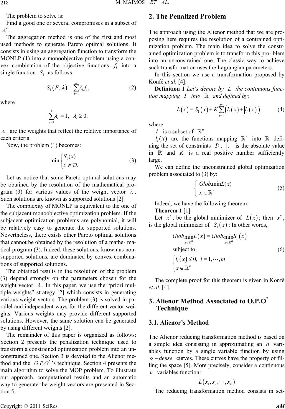

M. MAIMOS ET AL.
218
The problem to solve is:
Find a good one or several compromises in a subset of
n
.
The aggregation method is one of the first and most
used methods to generate Pareto optimal solutions. It
consists in using an agg r ega tion fun ctio n to transform the
MONLP (1) into a monoobjective problem using a con-
vex combination of the objective functions i
f
into a
single function 1 S as follows:

1=1
,= ,
k
ii
i
SF f 
 (2)
where
=1
=1, 0.
k
ii
i
 

i

are the weights that reflect the relative importance of
each criteria.
Now, the problem (1) becomes:
1()
min .
Sx
x


 (3)
Let us notice that some Pareto optimal solutions may
be obtained by the resolution of the mathematical pro-
gram (3) for various values of the weight vector

.
Such solutions are known as supported solu tions [2].
The complexity of MONLP is equivalent to the one of
the subjacent monoobjective optimization problem. If the
subjacent optimization problems are polynomial, it will
be relatively easy to generate the supported solutions.
Nevertheless, there exists other Pareto optimal solutions
that cannot be obtained by the resolution of a mathe- ma-
tical program (3). Indeed , these solutions, known as non-
supported solutions, are dominated by convex combina-
tions of suppo rted solutions.
The obtained results in the resolution of the problem
(3) depend strongly on the parameters chosen for the
weight vector

. In this paper, we use the “priori mul-
tiple weights” strategy [2] which consists in generating
various weight vectors. The problem (3) is solved in pa-
rallel and independent ways for the different vector wei-
ghts. Various weights may provide different supported
solutions. However, the same solution can be generated
by using different weights [2].
The remainder of this paper is organized as follows:
Section 2 presents the penalization technique used to
transform a constrained optimization prob lem into an un-
constrained one. Section 3 is devoted to the Alienor me-
thod and the * ..OPO’s technique. Section 4 presents the
main algorithm to solve the MOP problem. To illustrate
our approach, computational results and an automatic
way to generate the weight vectors are presented in Sec-
tion 5.
2. The Penalized Problem
The approach using the Alienor method that we are pro-
posing here requires the resolution of a contrained opti-
mization problem. The main idea to solve the constr-
ained optimization prob lem is to tran sfor m this pro- blem
into an unconstrained one. The classic way to achieve
such transform at i on uses t he Lagra n gi an paramete rs.
In this section we use a transformation proposed by
Konfé et al. [4]:
Definition 1 Let’s denote by L the continuous func-
tion mapping
I
into  and defined by:
 

1=1
=.
m
ii
i
LxSxKlxl x
 (4)
where
I
is a subset of n .
)(xli are the functions mapping n
 into  defi-
ning the set of constraints . |.| is the absolute value
in  and
K
is a real positive number sufficiently
large.
We can define the unconstrained global optimization
problem associated to (3) by:
.min ( )
n
GlobL x
x


 (5)
Indeed, we have the following theorem:
Theorem 1 [1]
Let
x

, be the global minimizer of

Lx; then
x

,
is the global minimizer of

1
Sx: In othe r wo rd s ,



1
=.
min min
subject to:
0, =1, ,
nn
xx
i
n
GlobL xGlobSx
lx im
x







(6)
The complete proof for this th eorem is given in Konfé
et al. [4].
3. Alienor Method Associa t ed t o O . P. O*
Technique
3.1. Alienor’s Method
The Alienor reducing transformation method is based on
a simple idea consisting in approximating an n vari-
ables function by a single variable function by using
dense


curves. These curves have the property of fil-
ling the space [5]. More precisely, consider a continuous
n variables function:


12
,,,
n
Lx xx
The reducing transformation method consists in set-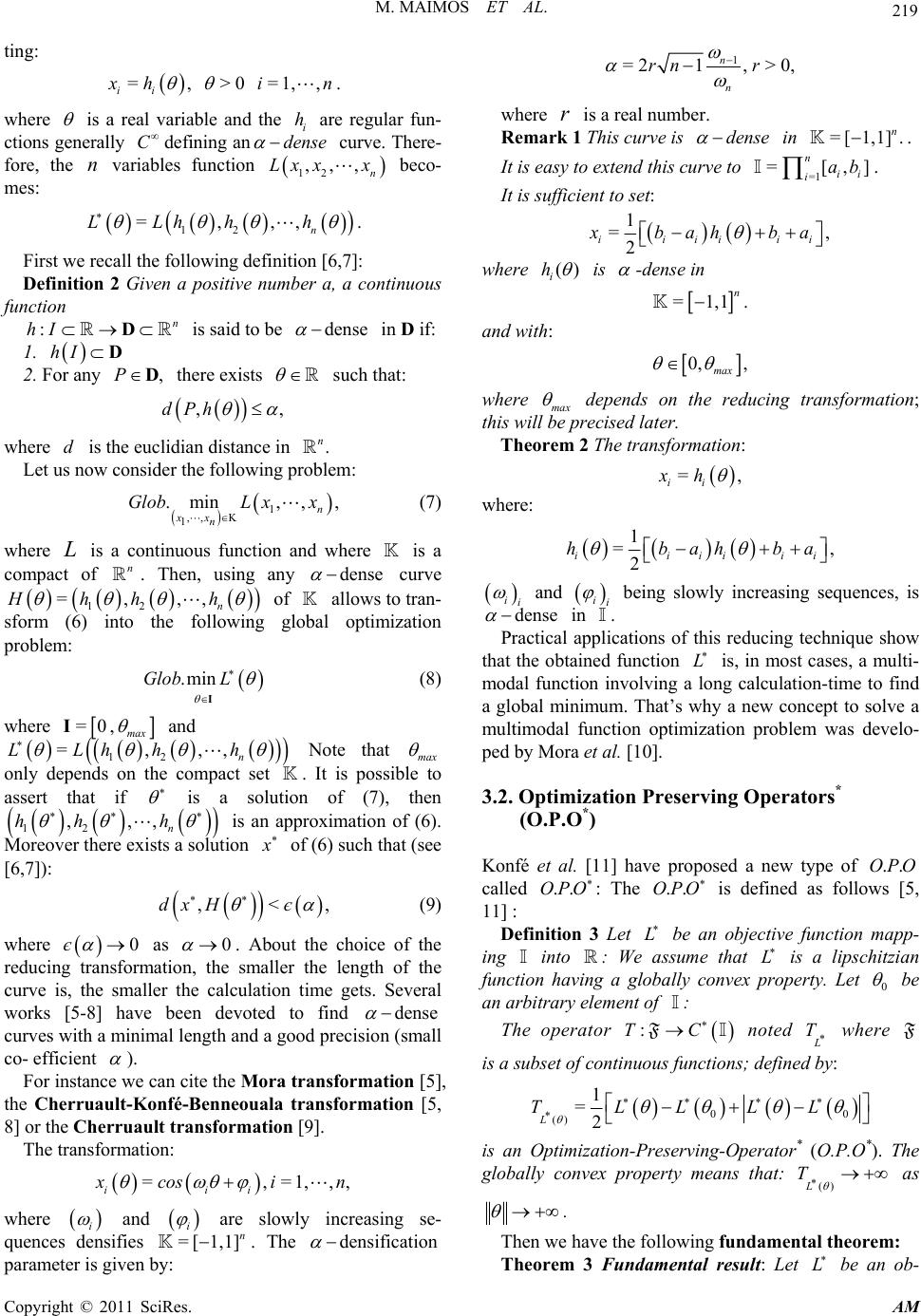

M. MAIMOS ET AL.
219
ting:

=, >0 =1,,
ii
x
hin  .
where

is a real variable and the i h are regular fun-
ctions generally Cdefining andense

 curve. There-
fore, the n variables function

12
,,,
n
Lx xx beco-
mes:
 

 
12
=,,,
n
LLhh h


.
First we recall the following definition [6,7]:
Definition 2 Given a positive number a, a continuous
function
:n hID is said to be dense

 in D if:
1.

hI D
2. For any ,PD there exists

 such that:
 
,,dPh

 
where d is the euclidian distance in .
n

Let us now consider the following problem:


1
,, K
1
.min,, ,
n
xx
n
GlobL xx

 (7)
where L is a continuous function and where  is a
compact of n
. Then, using any dense

 curve
  
12
=,,,
n
Hhh h

   of  allows to tran-
sform (6) into the following global optimization
problem:


.minGlob L



I
(8)
where


=0 , max  I and
 
 
12
=,,,
n
LLhh h 
 Note that max

only depends on the compact set . It is possible to
assert that if

 is a solution of (7), then
  
12
,,,
n
hh h  
 
 is an approximation of (6).
Moreover there exists a solution
x
 of (6) such that (see
[6,7]):
 

,<,dx Hє


 (9)
where

0є   as 0

. About the choice of the
reducing transformation, the smaller the length of the
curve is, the smaller the calculation time gets. Several
works [5-8] have been devoted to find dense


curves with a minimal length and a good precision (small
co- efficient

).
For instance we can cite the Mora transformation [5],
the Cherruault-Konfé-Benneouala transformation [5,
8] or the Cherruault transformation [9].
The transformation:
 
=, =1,,,
iii
x
cosi n  
where

i

and


i

are slowly increasing se-
quences densifies = [1,1]n
. The densification


parameter is given by:
1
=21,>0,
n
n
rn r




where
r
is a real number.
Remark 1 This curve is dense

 in = [1,1].
n
.
It is easy to extend this curve to =1 =[,]
n
ii
iab

.
It is sufficient to set:
 
1
=,
2
iiiiii
x
bah ba 





where ()
i
h

is

-dense in

=1,1.
n

and with:


0, ,
max
 
where max

depends on the reducing transformation;
this will be precised later.
Theorem 2 The transformation:

=,
ii
xh

where:
  
1
=,
2
iiiiii
hbahba 







ii

and


ii

being slowly increasing sequences, is
dense


in .
Practical applications of this reducing technique show
that the obtained function L is, in most cases, a multi-
modal function involving a long calculation-time to find
a global minimum. That’s why a new concept to solve a
multimodal function optimization problem was develo-
ped by Mora et al. [ 10 ] .
3.2. Optimization Preserving Operators*
(O.P.O*)
Konfé et al. [11] have proposed a new type of ..OPO
called ..OPO

: The ..OPO
 is defined as follows [5,
11] :
Definition 3 Let L

be an objective function mapp-
ing  into : We assume that L is a lipschitzian
function having a globally convex property. Let 0

be
an arbitrary element of :
The operator

:TC

F noted
L
T where F
is a subset of continuous functions; defined by:
   
00
()
1
=2
L
TLLLL

 
 






is an Optimization-Preserving-Operator* (O.P.O*). The
globally convex property means that: ()L
T

 as
 .
Then we have the following fundamental theorem:
Theorem 3 Fundamental result: Let L be an ob-

M. MAIMOS ET AL.
220
jective function, 0

is an arbitrary element of .
I
Let
S be the set of the solutions of:

=0.
L
T 
 (10)



If=, then=.
min
I
SGlobLL





In other words, if S contains a unique element, it is
the solution of the global minimization problem.
The complete proof for this theorem is given in [11].
To solve the global optimization problem (7), we use
the O.P.O* to find a unique 0

such that:

=0.
L
T


4. Algorithm
Now, we fully describe the algorithm we propose to
solve our initial problem (1).
The MOP problem to solve is:
 

12
,,,
"min" k
F
xfxfxfx
x






 (11)
Step 1: Use the weighted sum to aggregate the di-
fferent functions and therefore obtain the following ob-
jective function:
 
1=1
=.
k
ii
i
Sx fx 
 (12)
where
=1
=1, 0.
k
ii
i
 

Step 2: If the problem (1) is constrained, use the
penalization technique to define the multidimensional
function

Lx as in (13):
 

1=1
=,
m
ii
i
LxS xKl xl x
 (13)
given that


=0, =1,,
n
i
Dx lxim
; other-
wise, set
 
1
=LxS x.
Step 3: Use Alienor method to convert the multi-
dimensional function

Lx into a one variable function

L

 by setting:


=,
ii
xh

where:
  
1
=,
2
iiiiiii
hbacos ba 
 



0,2.

 
Step 4: O.P.O*
1) Initialization.
*Take an arbitrary initial point 0

in .
Use OPO*:



  


00
0=2
L
LL LL
T




 

to eliminate all local minima, i.e. solve



0=0.
L
T


2) *Now let i
S

be the set of solutions defined by:



()
=: =0
L
ii
ST

 
If


=
i
S



then stop:

 is a global minimizer of
F

; go to Step 3
*otherwise go to 3.
3) *update .
F
T
*Choose
ji
S



*then go to 2.
Step 5: Find:



1
=,=1,,
2
iiii ii
x
bahba in 









where= cos,=1,,
iii
hwin 



calculate .F


5. Computational Results
Computing environment:
We implemented the algorithm in Maple12 software on
an Intel Core2Duo CPU T5850 @2.16 GHz computer
with 4 GB RAM using a windows vista Service patch 2,
operating system.
In order to have graphical representations, we have
only considered bi-criteria problems with a large number
of variables.
5.1. Example 1: Zitzler’s Test Function
For the first example, we solve the well known Zitzler’s
test function. Note that this example is an unconstrained
MONLP problem, it has been solved in [12] and the true
Pareto fronts is fo und when

=1gX :


 

11
1
2
"min" g1
fX x
f
X
fX XgX








where
  
1
=2
9
=1 , =,,
1
n
in
i
g
XxXxx
n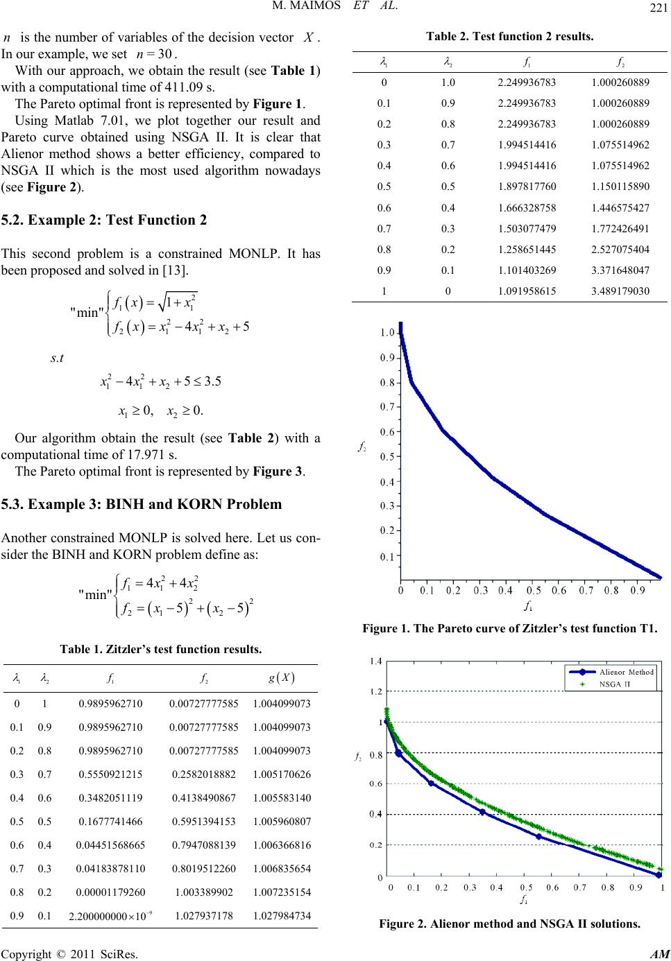


M. MAIMOS ET AL.
221
n is the number of variables of the decision vector
X
.
In our example, we set =30n.
With our approach, we obtain the result (see Table 1)
with a computational time of 411.09 s.
The Pareto optimal front is represented by Figure 1.
Using Matlab 7.01, we plot together our result and
Pareto curve obtained using NSGA II. It is clear that
Alienor method shows a better efficiency, compared to
NSGA II which is the most used algorithm nowadays
(see Figure 2).
5.2. Example 2: Test Function 2
This second problem is a constrained MONLP. It has
been proposed and solved in [13].


2
11
22
2112
1
"min" 45
fx x
fxxx x





s.t
22
112
453.5xxx
12
0, 0.xx
Our algorithm obtain the result (see Table 2) with a
computational time of 17.971 s.
The Pareto optimal front is represented by Figure 3.
5.3. Example 3: BINH and KORN Problem
Another constrained MONLP is solved here. Let us con-
sider the BINH and KORN problem define as:

22
112
22
21 2
44
"min" 55
fxx
fx x





Table 1. Zitzler’s test function results.
1

2

1
f
2
f


g
X
0 1 0.9895962710 0.00727777585 1.004099073
0.1 0.9 0.9895962710 0.00727777585 1.004099073
0.2 0.8 0.9895962710 0.00727777585 1.004099073
0.3 0.7 0.5550921215 0.2582018882 1.005170626
0.4 0.6 0.3482051119 0.4138490867 1.005583140
0.5 0.5 0.1677741466 0.5951394153 1.005960807
0.6 0.4 0.04451568665 0.7947088139 1.006366816
0.7 0.3 0.04183878110 0.8019512260 1.006835654
0.8 0.2 0.00001179260 1.003389902 1.007235154
0.9 0.1 9 2.200000000 10  1.027937178 1.027984734
Table 2. Test function 2 results.
1

2

1
f
2
f
0 1.0 2.249936783 1.000260889
0.1 0.9 2.249936783 1.000260889
0.2 0.8 2.249936783 1.000260889
0.3 0.7 1.994514416 1.075514962
0.4 0.6 1.994514416 1.075514962
0.5 0.5 1.897817760 1.150115890
0.6 0.4 1.666328758 1.446575427
0.7 0.3 1.503077479 1.772426491
0.8 0.2 1.258651445 2.527075404
0.9 0.1 1.101403269 3.371648047
1 0 1.091958615 3.489179030
Figure 1. The Pareto curve of Zitzler’s test function T1.
Figure 2. Alienor method and NSGA II solutions.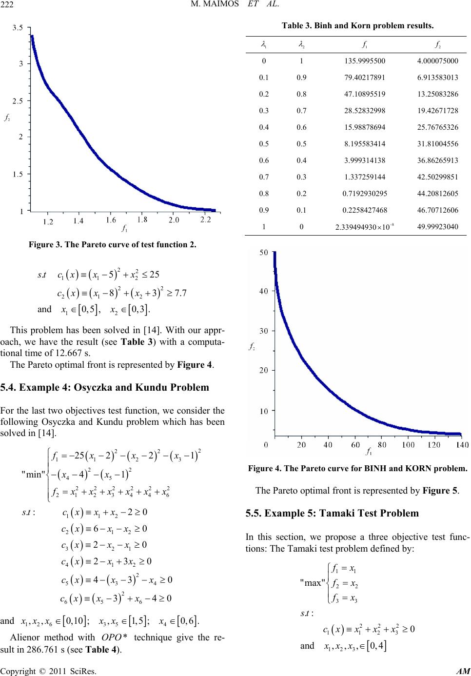

M. MAIMOS ET AL.
222
Figure 3. The Pareto curve of test function 2.
 
 
 
22
11 2
22
212
12
.525
837.7
and0,5,0,3 .
stc xxx
cx xx
xx
 


This problem has been solved in [14]. With our appr-
oach, we have the result (see Table 3) with a computa-
tional time of 12.667 s.
The Pareto optimal front is represented by Figure 4.
5.4. Example 4: Osyczka and Kundu Problem
For the last two objectives test function, we consider the
following Osyczka and Kundu problem which has been
solved in [14].
 
 




 


2 22
11 23
2 2
45
222222
2123446
112
212
321
412
2
534
2
65 6
25 221
"min"41
.:2 0
60
20
230
43 0
340
fx xx
xx
f xxxxxx
stc xxx
cxx x
cxx x
cxx x
cx xx
cx xx
 







 
 
 
 

and






12635 4
,,0,10;,1,5 ;0,6 .xx xxxx
Alienor method with *OPO technique give the re-
sult in 286.761 s (see Table 4).
Table 3. Binh and Korn problem results.
1

2

1
f
2
f
0 1 135.9995500 4.000075000
0.1 0.9 79.40217891 6.913583013
0.2 0.8 47.10895519 13.25083286
0.3 0.7 28.52832998 19.42671728
0.4 0.6 15.98878694 25.76765326
0.5 0.5 8.195583414 31.81004556
0.6 0.4 3.999314138 36.86265913
0.7 0.3 1.337259144 42.50299851
0.8 0.2 0.7192930295 44.20812605
0.9 0.1 0.2258427468 46.70712606
1 0 8 2.339494930 10  49.99923040
Figure 4. The Pareto curve for BINH and KORN problem.
The Pareto optimal front is represented by Figure 5.
5.5. Example 5: Tamaki Test Problem
In this section, we propose a three objective test func-
tions: The Tamaki test problem defined by:


11
22
33
222
1123
12 3
"max"
.:
0
and, , ,0,4
fx
fx
fx
st
cxxxx
xxx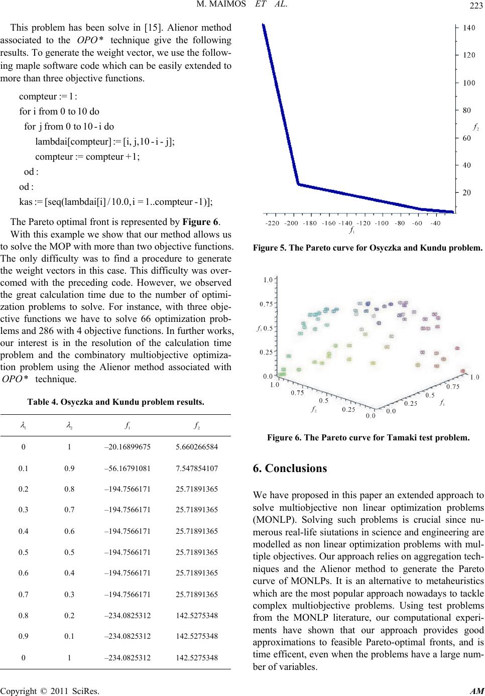










M. MAIMOS ET AL.
223
This problem has been solve in [15]. Alienor method
associated to the *OPO technique give the following
results. To generate the weight vector, we use the follow-
ing maple software code which can be easily extended to
more than three objective functions.
compteur :=1:
for ifrom 0to10 do
forj from0to10-ido
lambdai[compteur]:=[i, j,10-i-j];
compteur :=compteur +1;
od :
od :
kas:= [seq(lambdai[i]/10.0,i=1..compteur -1)];
The Pareto optimal front is represented by Figure 6.
With this example we show that our method allows us
to solve the MOP with more than two objective functions.
The only difficulty was to find a procedure to generate
the weight vectors in this case. This difficulty was over-
comed with the preceding code. However, we observed
the great calculation time due to the number of optimi-
zation problems to solve. For instance, with three obje-
ctive functions we have to solve 66 optimization prob-
lems and 286 with 4 objective functions. In further works,
our interest is in the resolution of the calculation time
problem and the combinatory multiobjective optimiza-
tion problem using the Alienor method associated with
*OPO technique.
Table 4. Osyczka and Kundu problem results.
1

2

1
f
2
f
0 1 –20.16899675 5.660266584
0.1 0.9 –56.16791081 7.547854107
0.2 0.8 –194.7566171 25.71891365
0.3 0.7 –194.7566171 25.71891365
0.4 0.6 –194.7566171 25.71891365
0.5 0.5 –194.7566171 25.71891365
0.6 0.4 –194.7566171 25.71891365
0.7 0.3 –194.7566171 25.71891365
0.8 0.2 –234.0825312 142.5275348
0.9 0.1 –234.0825312 142.5275348
0 1 –234.0825312 142.5275348
Figure 5. The Pareto curve for Osyczka and Kun du prob lem.
Figure 6. The Pareto curve for Tamaki test problem.
6. Conclusions
We have proposed in this paper an extended approach to
solve multiobjective non linear optimization problems
(MONLP). Solving such problems is crucial since nu-
merous real-life siutations in science and engineering are
modelled as non linear optimization problems with mul-
tiple objectives. Our ap proach relies o n aggreg ation tech-
niques and the Alienor method to generate the Pareto
curve of MONLPs. It is an alternative to metaheuristics
which are the most popular approach nowadays to tackle
complex multiobjective problems. Using test problems
from the MONLP literature, our computational experi-
ments have shown that our approach provides good
approximations to feasible Pareto-optimal fronts, and is
time efficent, even when the problems have a large num-
ber of variables.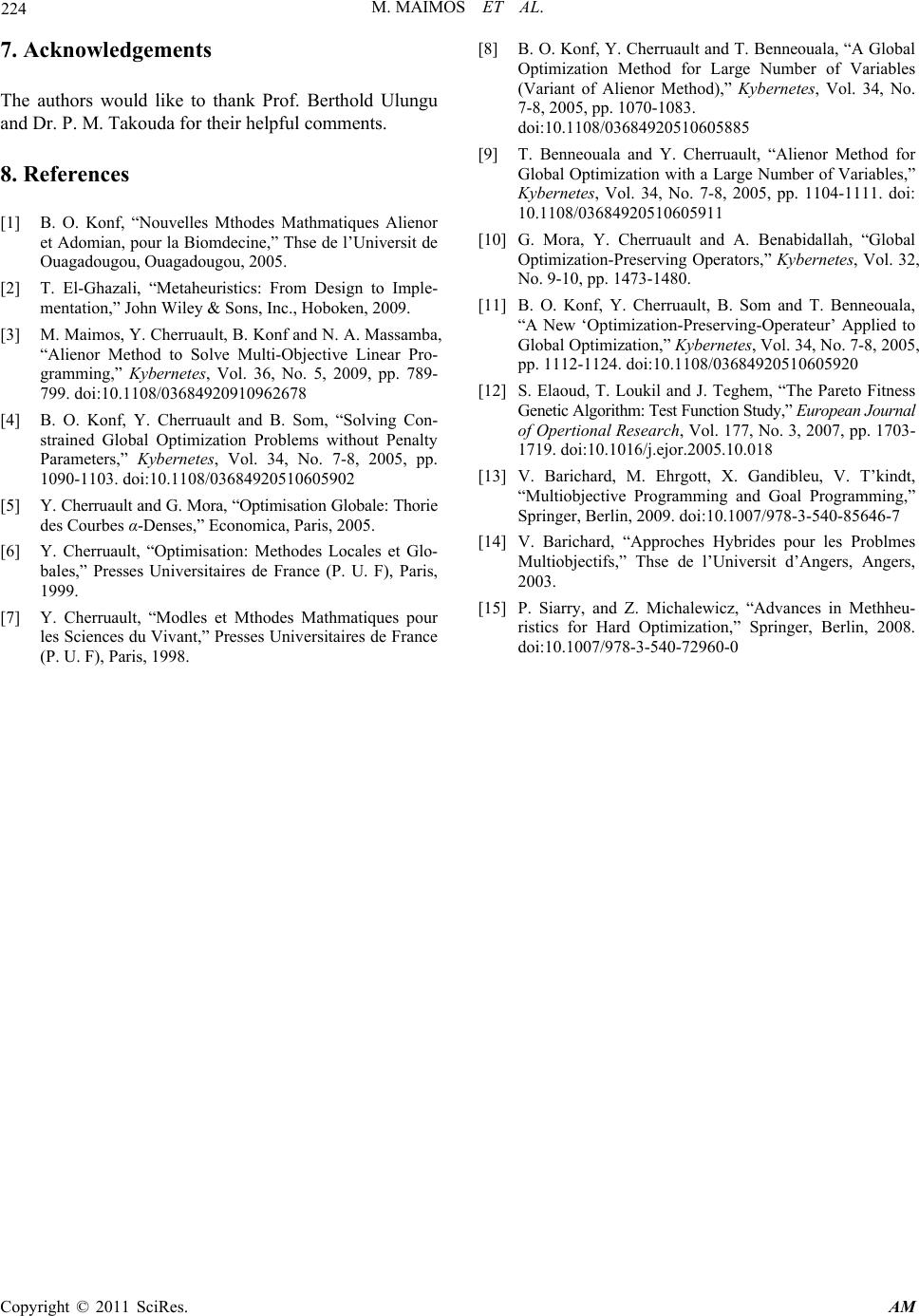

M. MAIMOS ET AL.
224
7. Acknowledgements
The authors would like to thank Prof. Berthold Ulungu
and Dr. P. M. Takouda for their helpful comments.
8. References
[1] B. O. Konf, “Nouvelles Mthodes Mathmatiques Alienor
et Adomian, pour la Biomdecine,” Thse de l’Universit de
Ouagadougou, Ouagadougou, 2005.
[2] T. El-Ghazali, “Metaheuristics: From Design to Imple-
mentation,” John Wiley & Sons, Inc., Hoboken, 2009.
[3] M. Maimos, Y. Cherruault, B. Konf and N. A. Massamba,
“Alienor Method to Solve Multi-Objective Linear Pro-
gramming,” Kybernetes, Vol. 36, No. 5, 2009, pp. 789-
799. doi:10.1108/03684920910962678
[4] B. O. Konf, Y. Cherruault and B. Som, “Solving Con-
strained Global Optimization Problems without Penalty
Parameters,” Kybernetes, Vol. 34, No. 7-8, 2005, pp.
1090-1103. doi:10.1108/03684920510605902
[5] Y. Cherruault and G. Mora, “Optimisation Globale : Thorie
des Courbes α-Denses,” Economica, Paris, 2005.
[6] Y. Cherruault, “Optimisation: Methodes Locales et Glo-
bales,” Presses Universitaires de France (P. U. F), Paris,
1999.
[7] Y. Cherruault, “Modles et Mthodes Mathmatiques pour
les Sciences du Vivant,” Presses Universitaires de France
(P. U. F), Paris, 1998.
[8] B. O. Konf, Y. Cherruault and T. Benneouala, “A Global
Optimization Method for Large Number of Variables
(Variant of Alienor Method),” Kybernetes, Vol. 34, No.
7-8, 2005, pp. 1070-1083.
doi:10.1108/03684920510605885
[9] T. Benneouala and Y. Cherruault, “Alienor Method for
Global Optimization with a Large Number of Variables,”
Kybernetes, Vol. 34, No. 7-8, 2005, pp. 1104-1111. doi:
10.1108/03684920510605911
[10] G. Mora, Y. Cherruault and A. Benabidallah, “Global
Optimization-Preserving Operators,” Kybernetes, Vol. 32,
No. 9-10, pp. 1473-1480.
[11] B. O. Konf, Y. Cherruault, B. Som and T. Benneouala,
“A New ‘Optimization-Preserving-Operateur’ Applied to
Global Optimization,” Kybernetes, Vol. 34, No. 7-8, 2005,
pp. 1112-1124. doi:10.1108/03684920510605920
[12] S. Elaoud, T. Loukil and J. Teghem, “The Pareto Fitness
Genetic Alg or ithm: Test Function Study,” European Journal
of Opertional Research, Vol. 177, No. 3, 2007, pp. 1703-
1719. doi:10.1016/j.ejor.2005.10.018
[13] V. Barichard, M. Ehrgott, X. Gandibleu, V. T’kindt,
“Multiobjective Programming and Goal Programming,”
Springer, Berlin, 2009. doi:10.1007/978-3-540-85646-7
[14] V. Barichard, “Approches Hybrides pour les Problmes
Multiobjectifs,” Thse de l’Universit d’Angers, Angers,
2003.
[15] P. Siarry, and Z. Michalewicz, “Advances in Methheu-
ristics for Hard Optimization,” Springer, Berlin, 2008.
doi:10.1007/978-3-540-72960-0