Energy and Power Engineering, 2013, 5, 1277-1283
doi:10.4236/epe.2013.54B242 Published Online July 2013 (http://www.scirp.org/journal/epe)
A Fast Extraction Method in the Applicaton of UHV
Transmission Line Fault Location*
Li Wang1,2, Jiale Suonan1, Zaibin Jiao1
1Department of Electrical Engineering, Xi'an Jiaotong University, Xi’an, China
2Department of Technology Center , XJ Group Limited Company, Xuchang, China
Received February, 2013
ABSTRACT
To aim at the distribution parameter characteristics of UHV transmission line, this paper presents a fast extraction
method (FE) to extract the accurate fundamentals of current and voltage from the UHV transmission line transient
process, and locates the fault by utilizing two-end unsynchronized algorithm. The simulation result shows that this
method has good performance of accuracy and stability, and has better location precision by comparing with results of
one cycle Fourier algorithm. Therefore the method can efficiently improve the precision of fault location during the
transient process, and makes the error of location results less than 0.5%.
Keywords: UHV; Fast Extraction Method; Matrix Pencil; Transient Process; Fault Location
1. Introduction
Recently, with the development of communication tech-
nology and the improvement of electric power automa-
tion system, two-terminal fault location method [1-6] has
been gradually popularized in the power system. With
the increasing of UHV long transmission line, two-ter-
minal fault location method that employs the accurate
distributed parameter model and need not synchronized
data of two-terminal will be applied extensively. Com-
pared with HV and EHV transmission line, UHV trans-
mission line has the characteristics of large transmission
capacity, long transmission distance, smaller wave im-
pedance and larger distributed capacitance, so the fault
transient process will be more complicated, and accu-
rately acquiring of fault electric quantity would be diffi-
cult. Most of existing location algorithms based on pha-
sor method. In the transient process of UHV AC trans-
mission system, the decaying DC offset of fault current
and the decaying DC offset of fault voltage introduced by
CVT extend the convergence time of the traditio nal Fou-
rier algorithm, decrease the accuracy of algorithm, and
also reduce the precision of electric quantities in the fau lt
transient process.
In order to remove the influence of decaying DC offset,
many domestic and foreign scholars have proposed some
improved algorithms, such as difference Fourier algo-
rithm[7] and parallel compensatio n method [8]. Although
difference Fourier algorithm can suppress the DC offset
in a certain extent, it cannot remove the decaying DC
offset; meanwhile it also amplifies the content of har-
monics. Parallel compensation method required the prior
knowledge regarding the time constant of the DC offset,
so it is difficult to realize in practical engineering . On the
premise of relay protection rapid action, the present algo-
rithm has a high demand of rapidity, which will sacrifice
some accuracy and stability. But the UHV transmission
line require not only th e higher accuracy of fault location,
but also protection quick trip over ten milliseconds, then
the voltage and current data window would less th an one
cycle. In order to calculate fault location fast and accu-
rately, it is important to introduce a new phasor extrac-
tion algorithm.
Based on Matrix Pencil method [9-12], the Fast Ex-
traction method [13] is established by using matrix simi-
lar transformation and QR Factorization. It can quickly
extract the fundamental frequency component of UHV
transmission line, and remove the effect of decaying DC
offset and high order harmonic component of the tran-
sient process. This paper uses the Fast Extraction method
to identify the fundamental component of fault compo-
nent within 20 ms, and applies the fundamental to
two-terminal fault location scheme for fault location,
which greatly improves the accuracy of fault location
during transient process, and has a good application
prospect.
*The research presented in this paper is supported by National Natural
Science Foundation of China (51037005) and Specialized Research
Fund for the Doctoral Program of Higher Education (2011020111
0056).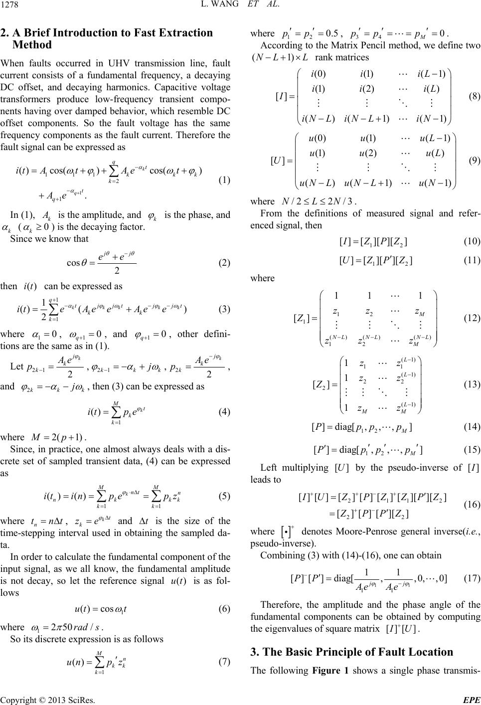

L. WANG ET AL.
1278
2. A Brief Introduction to Fast Extraction
Method
When faults occurred in UHV transmission line, fault
current consists of a fundamental frequency, a decaying
DC offset, and decaying harmonics. Capacitive voltage
transformers produce low-frequency transient compo-
nents having over damped behavior, which resemble DC
offset components. So the fault voltage has the same
frequency components as the fault current. Therefore the
fault signal can be expressed as
1
111
2
1
() cos()cos()
.
k
q
q
t
kk
k
t
q
it AtAet
Ae


k








 

 (1)
In (1), k
A
is the amplitude, and k

is the phase, and
k

(0
k

) is the decaying factor.
Since we know that
cos 2
j
j
ee





 (2)
then can be expressed as ()it
1
1
1
() ()
2kkk k
q
tjjt jjt
kk
k
iteAeeAee
 



k

(3)
where 10

, 10
q

, and 10 q

, other defini-
tions are the same as in (1).
Let 21 2
k
j
k
k
A
e
p

,21kk
jk


 ,22
k
j
k
k
Ae
p


,
and 2kk jk

    , then (3) can be expressed as
1
() k
Mt
k
k
it pe


 (4)
where . 2( 1)Mp
Since, in practice, one almost always deals with a dis-
crete set of sampled transient data, (4) can be expressed
as
11
() ()k
MM
nt n
nk
kk
it inpepz
 

 

kk
t
(5)
where n, and is the size of the
time-stepping interval used in obtaining the sampled da-
ta.
tn kt
k
ze
 
t
In order to calculate the fundamental component of the
input signal, as we all know, the fundamental amplitude
is not decay, so let the reference signal is as fol-
lows ()ut
1
() cosut t

 (6)
where 1250 /rad s

 .
So its discrete expression is as follows
(7)
where ,
Acco
1
() Mn
kk
k
unp z



12
0.5pp


rding to the Ma3
pp p
 
 
trix Penc
40 M.
il method, we define two
(1)NL L

 rank mtrices
(8)
(9)
where
a
(0)(1)( 1)
(1) (2)
ii iL
ii
 


( )
[]
()(1) (1)
iL
I
iN LiN LiN



 




(0)(1)( 1)
(1)(2)( )
[]
()( 1)(1)
uu uL
uu uL
U
uN LuN LuN
 




 





/22 /3NLN

.
From the definitions of measured signal and refer-
hen enced signal, t
12
[][][ ][]
I
ZPZ

(10)
12
[][][][]UZPZ


(11)
where
(12)
(13)
12
1
() ()()
12
11
[] M
NL NLNL
M
zz z
Z
zz z
 











1
(1)
11
(1)
22
2
(1)
1
1
[]
1
L
L
L
MM
zz
zz
Z
zz














12
[] diag[,,,]
M
Pppp

 (14)
(15)
Left multiplying by the pseudo
12
[]diag[,,,]
M
Pppp
 

[]U -inverse of []
I
leads to
2112
[][]][ ][][][][]
22
[
[][][][]
I
UZPZZPZ


 (1)
ZP PZ


6
where




o-invedenotes Moore-Penrose general inv pseudrse).
bining
erse(i.e.,
Com (3) with (14)-(16), one can obtain
11
11
] diag[,,0,,0]
 (17)
Therefore, the amplitude and the phase angl
fundamental components can be obtained by co
the eige
11
[][PP
jj
Ae Ae


e of the
mputing
nvalues of square matrix [][ ]
I
U
3. The Basic Principle of Fault Location
.
The following Figure 1 shows a single phase transmis-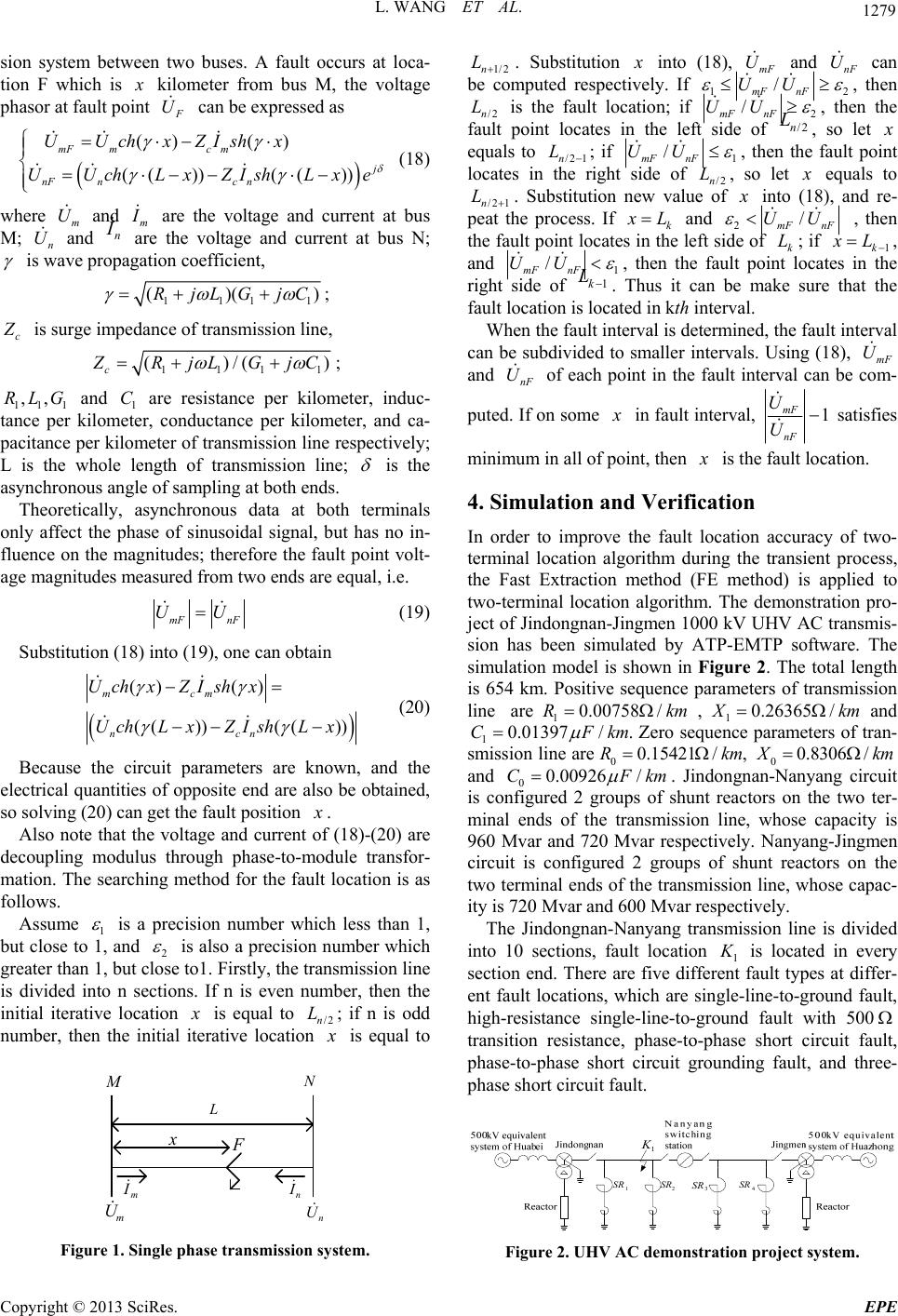

L. WANG ET AL. 1279
sion system between two buses. A fault occurs at loca-
tion F which is
x
kilometer from bus M, the voltage
phasor at fault point
F
U
 can be expressed as

) ()
(( ))(())
mFmc m

(
j
nFnc ne
UUchxZIshx
UUch LxZIsh Lx



 


 
 



(18)
where and
m
U

m
I
 are the voltage and current
M; d at bus
n anU
n
I
 are the voltage and current at bus N;

is w propagion coefficient, aveat
1111
()()RjLGjC  ;
c
Z
is surge impedance of transmission line,
1111c()/()
Z
RjLGjC   
-
r kiloter, conductance per kilomr, and ca-
;
11 1
,,R
tance pe
pacitance per kilo
LG and C are resistance per kilometer, induc
1
me ete
meter of transmission line respectively;
L is the whole length of transmission line;

is the
asynchronous angle of sampling at both ends.
Theoretically, asynchronous data at both terminals
only affect the phase of sinusoidal signal, but has no in-
fluence on the magnitudes; therefore the fault point volt-
age magnitudes measured from two ends are equal, i.e.
mF nF
UU

(19)
Substitution (18) into (19), one can obtain

() ()
(( ))(( ))
nc
n
Uch xZIshx
UchLxZIshLx



 

(20)
Because the circuit parameters are known
electrical quantities of opposite end are also be obtained,
so
mcm

, and the
solving (20) can get the fault position
x
.
Also note that the voltage and current of (18)-(20) are
decoupling modulus through phase-to-module transfor-
mation. The searching method for the fault location is as
follows.
Assume 1

is a precision number which less than 1,
but close to 1, and 2

is also a precision number which
greater than but close to1. Firstly, the transmission line
is divided into n sections. If n is even number, then the
initial iterative location
1,
x
is equal to /2n L; if n is odd
number, then the initial iterative location
x
is equal to
F
x
L
m
I

n
I

n
U

m
U

M
N
Figure 1. Single phase transmission system.
. Substitution
1/2n
L
x
into (18), and can
puted re. If mF
U

nF
U

be comspectively 12 /
mF
UU
nF

 
 , then
is the fault location; if
/2n
L 2 /
mF nF
UU


 he
point locates in the left side of , then t , so letfault /2n
L
x
equals to /2 1n
L

; if 1 /
mF nF
UU


 , thee fa
e right side of , so let
n thult point
locates in th/2n L
x
equals to
/2 1n
L

. Substitution new value of
x
into (18), and re-
peat the process. If k
x
L

and 2/
mF nF
UU  
f L

, then
the fault point locates in the left sidek; if 1k o
x
L


,
and 1
/
mF nF
UU


 , then the fault in the
right side of 1k
Lpoint locates

. Thus it care that the
fault location is located in kth interval.
When the fault interined, the fault interval
can be subdivided to smaller intervals. Using (18), mF
U

and nF
U
 of each point in the fault interval can be com-
puted. If on some
n be ma
val is determ
ke su
x
in faval,ult inter 1
mF
nF
U
Uatisfies
minioint, then


 s
mum in all of p
x
is the fault location.
4. Simulation and Verification
In order to improve the fault location accuracy of two-
termil location algorithm during the transient process,
the Fast Extraction method (FE methos applied to
na d) i
emonstra
ject of Jindongnan- Jingmen 1000 kV UHV AC transmis-
he
simulation model is shown in Figure 2. The total length
s of transmission
two-terminal location algorithm. The dtion pro-
sion has been simulated by ATP-EMTP software. T
is 654 km. Positive sequence parameter
line are0.00758 /Rkm
1

,0.26
1365 /
X
kmand
10.01397/ .CFkm


Zero sequence parameters of tran-
smission line are 00.15421 /,Rkm

 00.8306 /
X
km
and 00.00926 /CFkm


. Jindongnan-Nanyang circuit
is configured 2 groups of shunt reactors on the two ter-
minal ends of the transmission line, whose capacity is
960 Mvar and 720 Mvar respectively. Nanyang-Jingmen
circuit is configured 2 groups of shunt reactors on the
two terminal ends of the transmission line, whose capac-
ity is 720 re
nyang transmission line is divided
into 10 sections, 1
Mvar and 600 Mvar spectively.
The Jindongnan-Na
fault location
K
is located in every
section end. There are five different fault types at differ-
ent fault locations, which are single-line-to-ground fault,
high-resistance single-line-to-ground fault with 500

transition resistance, phase-to-phase short circuit fault,
phase-to-phase short circuit grounding fault, and three-
phase short circuit fault.
1
K
1
SR
2
SR
3
SR
4
SR
Figure 2. UHV AC demonstration project system.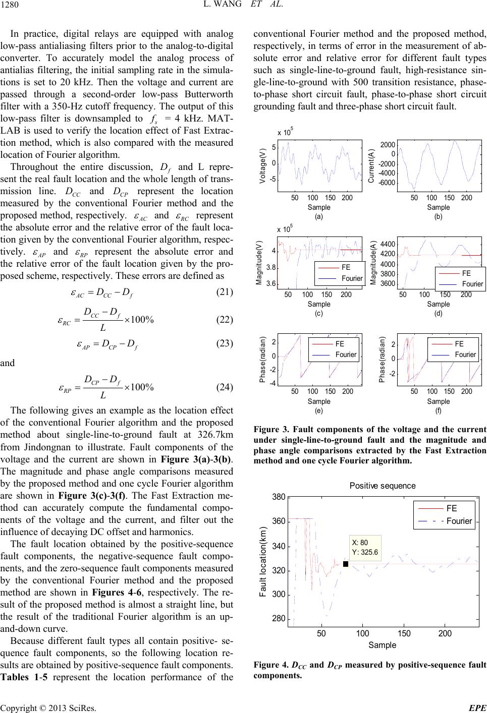

L. WANG ET AL.
1280
In practice, digital relays are equipped with analog
low-pass antialiasing filters prior to the analog-to-digital
onverter. To accurately model the analog process of
antialias filtering, the initial sampling rate in the simula-
tions is set to 20 kHz. Then the voltage and current are
passed through a second-order low-pass Butterworth
filter with a 350-Hz cutoff frequency. The output of this
low-pass filter is downsampled to
c
s
f = 4 kHz. MAT-
LAB
tio is used to verify the location effect of Fast Extrac- n method, which is also compared with the measured
location of Fourier algorithm.
Throughout the entire discussion,
f
D and L repre-
sent the real fault location and the whole length of trans-
mission line. CC
D and CP D represent the location
measured by the conventional Fourier method and the
proposed method, respectively. AC

and
R
C

represent
the absolute error and the relative error of the fault loca-
tion given by the conventional Fourier algorithm, respec-
tively. AP

and
R
P

represent the absolute error and
the relative error of the fault location given by the pro-
posed scheme, respectively. These errors are defined as
AC CC f
DD

 (21)
100%
CC f
RC
DD
L



(22)
AP CP f
DD

 (23)
and
100%
CPf
RP
DD
L


 (24)
The following gives an examp
of the conventional Fourier algorithm and the proposed
method about single-line-to-ground
from Jindongnan to illustrate. Fault components of the
voltage and the current are show
magnitude and phase angle comparisons measured
e proposed method and one cycle Fourier algorithm
are shown in Figure 3(c)-3(f). The F
thod can accurately compute the fundamental c
ne
t fault, phase-to-phase short circuit
gr
le as the location effect
fault at 326.7km
n in Figure 3(a)-3(b).
The
by thast Extraction me-
ompo-
nts of the voltage and the current, and filter out the
influenc e of decaying DC offset and ha rmonics.
The fault location obtained by the positive-sequence
fault components, the negative-sequence fault compo-
nents, and the zero-sequence fault components measured
by the conventional Fourier method and the proposed
method are shown in Figures 4-6, respectively. The re-
sult of the proposed method is almost a straight line, but
the result of the traditional Fourier algorithm is an up-
and-down curve.
Because different fault types all contain positive- se-
quence fault components, so the following location re-
sults are obtained by positive-sequence fault components.
Tables 1-5 represent the location performance of the
conventional Fourier method and the proposed method,
respectively, in terms of error in the measurement of ab-
solute error and relative error for different fault types
such as single-line-to-ground fault, high-resistance sin-
gle-line-to-ground with 500 transition resistance, phase-
to-phase short circui
ounding fault and three-phase short circuit fault.
50 100150 200
-5
0
5
x 10
5
Sample
(a)
Voltage(V)
50 100 150200
3.6
3.8
4
x 10
5
Sample
(c)
M agnitude(
V)
FE
Fouri er
50 100 150 200
-4
-2
0
2
Sample
(e)
Phase(radian)
FE
Fourier
50100 150 200
-6000
-4000
-2000
0
2000
Sample
(b)
Current(A)
50 100 150 200
3600
3800
4000
4200
4400
Sample
(d)
Ma gnitude(A)
FE
Fouri er
50 100 150200
-2
0
2
Sample
(f)
Phase(radian)
FE
Fourier
Figure 3. Fault components of the voltage and the current
under single-line-to-ground fault and the magnitude and
phase angle comparisons extracted by the Fast Extraction
method and one cycle Fourier algorithm.
50100150200
280
300
320
340
360
380
Sample
km)
P ositi ve sequence
FE
Fourier
Fault location(
X: 80
Y: 325.6
Figure 4. DCC and DCP measured by positive-sequence fault
components.

L. WANG ET AL. 1281
Ta 2. Lesh sin-
ground fault
50 100 150 200
260
280
300
320
340
360
380
X: 80
Y: 325.6
Sample
Fault l oc ati on(k m)
Negati ve sequenc e
FE
Fourier
Figure 5. DCC and DCP measured by negative -sequence fau
lt components.
50100150200
260
280
300
320
340
360
X: 80
Y: 326.8
Sample
Fault location(km)
Zero sequence
FE
Fourier
Figure 6. DCC and DCP measured by zero-sequence faul
able 1. Location results of single-line-to-ground fault using
sequence fault fundamental components computed
by Fast Extraction method and one cycle Fourier algorithm.
Df (km) DCC (km) εRC (%) DCP (km) εRP (%)
t
components.
T
positive
0 [0.0,11.7] [0.00,3.22][1.30,1.60] [0.36,0.44]
36.3 [30.4,46.7] [-1.63,2.87][37.3,37.5] [0.28,0.33]
72.6 [65.0,84.0] [-2.09,3.14][73.2,73.5] [0.17,0.25]
108.9 [102.2,117.8] [-1.85,2.45][109.2,109.4] [0.08,0.14]
145.2 [140.3,151.3] [-1.35,1.68][145.2,145.3] [0.00,0.027]
181.5 [180.9,181.5] [-0.17,0.00][181.1,181.2] [-0.11,-0.08]
[3] [3 [-]
217.8 [211.4,221.6] [-1.76,-1.05][217.1,217.1] [-0.19,-0.17]
254.1 [244.8,260.5] [-2.56,1.76][253.0,253.1] [-0.30,-0.28]
290.4 [278.8,297.9] [-3.20,2.07][288.9,289.0] [-0.41,-0.39]
326.7 [315.2,333.6] [-3.17,1.9] [325.4,325.6] [-0.36,-0.30]
363 49.9,363.0[-3.61,0.0]61.5,361.6]0.41,-0.39
bleocation r
with 500
ults of higresistance gle-line-to

using positive seque
fundamenntt n
method and one cycle Fourier algorithm.
nce fault
tal compoents compued by FasExtractio
Df (km)DCC (km) εRC (%) DCP (km) εRP (%)
0 [0.00,17.9][0,4.93] [1.40,1.60] [0.39,0.44]
36.3 [34.4,51.0][-0.52,4.05] [37.3,37.6] [0.28,0.36]
72.6 [70.3,83.9][-0.63,3.11] [73.2,73.5] [0.17,0.25]
[-
3.1] [-0.33,-0.28]
[2][- [2] [-]
3[[-] [
[[
108.9[105.7,116.8][-0.88,2.18] [109.2,109.3] [0.08,0.11]
145.2[141.8,149.9][-0.94,1.29] [145.2,145.3] [0.00,0.027]
181.5[181.1,181.3]0.11,-0.06] [181.1,181.2] [-0.11,-0.08]
217.8[212.4,220.4][-1.49,0.72] [217.0,217.1] [-0.22,-0.19]
254.1[245.7,256.6][-2.31,0.69] [252.9,25
290.478.6,291.93.25,0.41] 88.9,289.0 0.41,-0.39
26.7312.2,328.7]3.99,0.55325.4,325.7][-0.36,-0.28]
363 345.2,363.0][-4.90,0.00] 361.5,361.6][-0.41,-0.39]
Tab shor
fault using posiquel cts
cethyr
algorithm.
)
le 3. Location results of phase-to-phaset circuit
tive se
d by Fast Exnce fault fundame raction metnta od and one componen cle Fourieomput
Df (kmDCC (km) εRC (% ) DCP (km) εRP (%)
0 [0.0,9.2] [0,2.53] 1.5 0.41
36.3 [29.9,45.2]
]
3]
2 [141]
181.5 [180.8,181.5][-0.19,0.00] 181.2 -0.08
[2.][-9 [ [-1]
326.7 [312.8,332.8][-3.83,1.68] 325.6 -0.30
363 [354.2,363.0][-2.42,0.00] 361.5 -0.41
[-1.76,2.45]37.4 0.30
72.6 [67.6,79.3[-1.38,1.85]73.4 0.22
108.9 [106.4,112.[-0.69,0.94]109.3 0.11
145.3.3,147.[-0.52,0.52]145.2 0
217.8 [215.7,218.6][-0.58,0.22] 217.1 -0.19
254.1 [250.5,255.5][-0.99,0.39] 253 -0.30
290.4 835,294.41.0,1.10]288.9,289]0.4,-0.39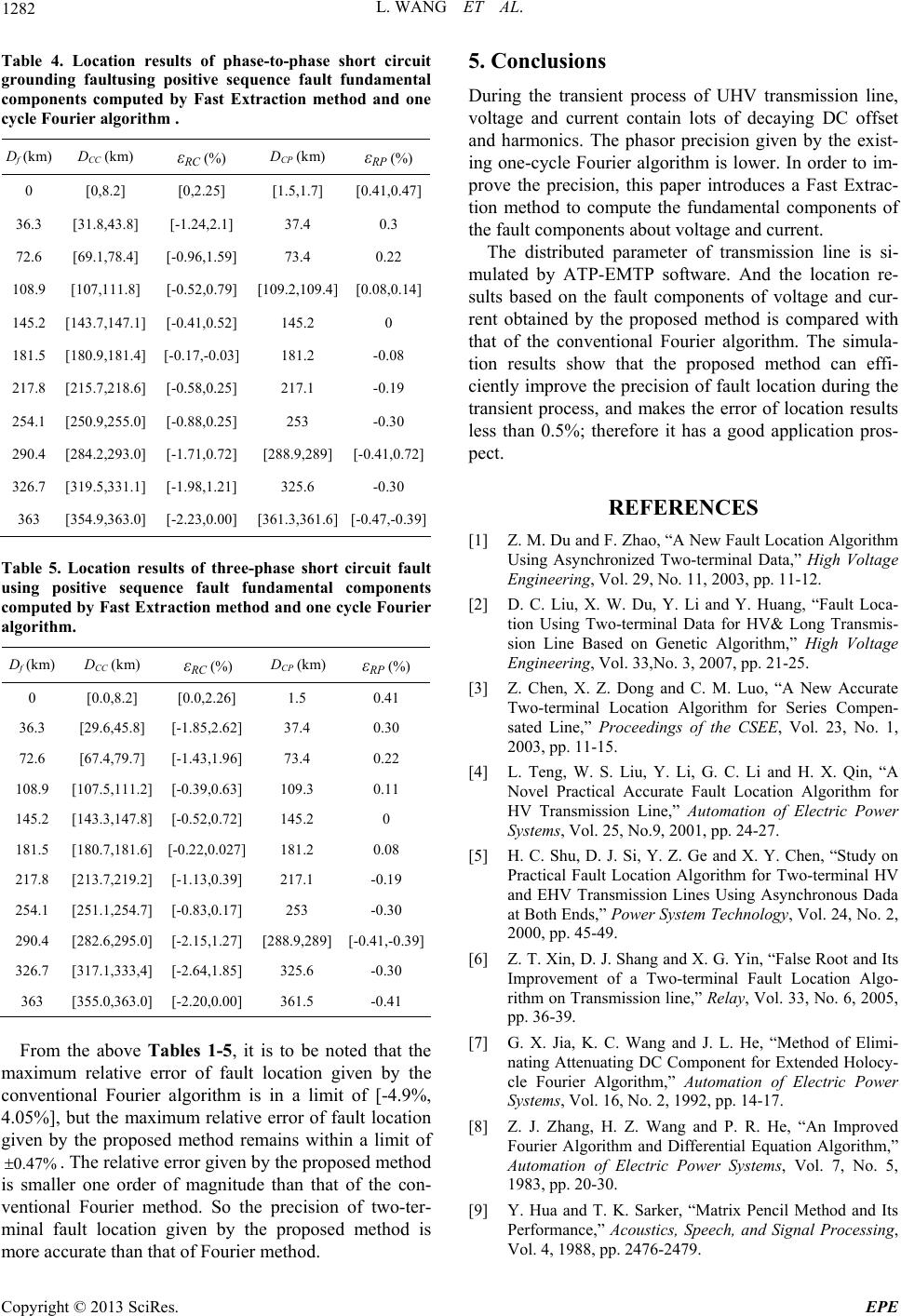

L. WANG ET AL.
1282
Tabu -to-phase shoruit
grng puenlt funntal
components computed byethod and one
cy urim
D) )
le 4. Locat
oundi ion res faultusing lts of phase ositive seqt circ damece fau
Fast Extract
. ion m cle Foer algorith
f (km) DCC (km) εRC (%) DCP (kmεRP (%
0 [0,8.2] [0,2.25] [1.5,1.7] [0.4.47]1,0
36.3 [31.8,43.8] [-1.24,2.1] 37.4 0.3
72.6 [69.1,78.4] [-0.96,1.59]73.4 0.22
108.9 [107,111.8] [-0.52,0.79][109.2,109.4] [0.08,0.14]
1 [1
1 [1[-
2 [2
254.1 [250.9,255.0] [-0.88,0.25]253 -0.30
45.2 43.7,147.1] [-0.41,0.52]145.2 0
81.5 80.9,181.4] 0.17,-0.03] 181.2 -0.08
17.8 15.7,218.6] [-0.58,0.25]217.1 -0.19
290.4 [284.2,293.0] [-1.71,0.72][288.9,289] [-0.41,0.72]
326.7 [319.5,331.1] [-1.98,1.21]325.6 -0.30
363 [354.9,363.0] [-2.23,0.00][361.3,361.6] [-0.47,-0.39]
Lesulee-pht cirlt
using positivequenco
computed bExtrathod cy
a hm
D) D) ε
Table 5.ocation rts of thrase shorcuit fau
se
y Fast e fault fundame ction mental c and onemponents cle Fourier
lgorit.
f (kmDCC (km) εRC (%) CP (kmRP (%)
0 [0.0,8.2] [0.0,2.26] 1.5 0.41
36.3 [29.6,45.8] [-1.85,2.62] 0.
254.1 [251.1,254.7] [-0.83,0.17] 253 -0.30
37.4 30
72.6 [67.4,79.7] [-1.43,1.96] 73.4 0.22
108.9 [107.5,111.2] [-0.39,0.63]109.3 0.11
145.2 [143.3,147.8] [-0.52,0.72]145.2 0
181.5 [180.7,181.6][-0.22,0.027]181.2 0.08
217.8 [213.7,219.2][-1.13,0.39]217.1 -0.19
290.4 [282.6,295.0][-2.15,1.27] [288.9,289] [-0.41,-0.39]
326.7 [317.1,333,4] [-2.64,1.85] 325.6 -0.30
363 [355.0,363.0] [-2.20,0.00] 361.5 -0.41
From the above Tables 1-5, it is to be noted that the
mm errot lvee
contioner aimit of%
4.05xime error of fault lo
gi tedmaiithin a of
T eby toposed method
isleof m that of ton-
ventete pon of t
mahe ed med is
more accurate than that of Fourier method.
5 c
During tpHsmissne,
voltage acof ing Dset
and harmhsion thist-
in-cr so
prove thethtro Fastac-
tioethuamompoof
he fat comnrrent.
mission Lines Using Asynchronous Dada
at Both Ends,” Power System Technology, Vol. 24, No. 2,
2000, pp. 45-4
aximurelative r of faulocation gin by th
,
[
ven
%], bual Fouri t the malgorithm is in um relativ a l [-4.9 cation
[8]
ven byhe propos method rens w limit
0.47%.he relativerror given he pr
smal
ionalr one order Fourier magnitude hod. So than th recisi he c wo-ter-
[9] Y. Hua and T. K. Sarker, “Matrix Pencil Method and Its
Performance,” Acoustics, Speech, and Signal Processing,
Vol. 4, 1988, pp. 2476-2479.
inal fult location given by tpropostho
. Conlusions
he transient rocess of UV tranion li
nd current
onics. The pontain lots asor precidecay given byC off e ex
g oneycle Fouriealgorithm i lower. In rder to im-
precision, is paper induces a Extr
n m
ul od to comp ponents ate the fund bout voltage aental c d cunents tThe distributed parameter of transmission line is si-
mulated by ATP-EMTP software. And the location re-
sults based on the fault components of voltage and cur-
rent obtained by the proposed method is compared with
that of the conventional Fourier algorithm. The simula-
tion results show that the proposed method can effi-
ciently improve the precision of fault location during the
transient process, and makes the error of location results
less than 0.5%; therefore it has a good application pros-
pect.
REFERENCES
[1] Z. M. Du and F. Zhao, “A New Fault Location Algorithm
Using Asynchronized Two-terminal Data,” High Voltage
Engineering, Vol. 29, No. 11, 2003, pp. 11-12.
[2] D. C. Liu, X. W. Du, Y. Li and Y. Huang, “Fault Loca-
tion Using Two-terminal Data for HV& Long Transmis-
sion Line Based on Genetic Algorithm,” High Voltage
Engineering, Vol. 33,No. 3, 2007, pp. 21-25.
[3] Z. Chen, X. Z. Dong and C. M. Luo, “A New Accurate
Two-terminal Location Algorithm for Series Compen-
sated Line,” Proceedings of the CSEE, Vol. 23, No. 1,
2003, pp. 11-15.
[4] L. Teng, W. S. Liu, Y. Li, G. C. Li and H. X. Qin, “A
Novel Practical Accurate Fault Location Algorithm for
HV Transmission Line,” Automation of Electric Power
Systems, Vol. 25, No.9, 2001, pp. 24-27.
[5] H. C. Shu, D. J. Si, Y. Z. Ge and X. Y. Chen, “Study on
Practical Fault Location Algorithm for Two-terminal HV
and EHV Trans
9.
[6] Z. T. Xin, D. J. Shang and X. G. Yin, “False Root and Its
Improvement of a Two-terminal Fault Location Algo-
rithm on Transmission line,” Relay, Vol. 33, No. 6, 2005,
pp. 36-39.
7] G. X. Jia, K. C. Wang and J. L. He, “Method of Elimi-
nating Attenuating DC Component for Extended Holocy-
cle Fourier Algorithm,” Automation of Electric Power
Systems, Vol. 16, No. 2, 1992, pp. 14-17.
Z. J. Zhang, H. Z. Wang and P. R. He, “An Improved
Fourier Algorithm and Differential Equation Algorithm,”
Automation of Electric Power Systems, Vol. 7, No. 5,
1983, pp. 20-30.

L. WANG ET AL.
1283
Method for Es-[10] Y. Hua and T. K. Sarker, “Matrix Pencil
timating Parameters of Exponentially Damped/ undamped
sinusoids in Noise,” IEEE Transaction on Acoustics,
Speech, and Signal Processing, Vol. 38, No. 5, 1990, pp.
814-824. doi:10.1109/29.56027
[11] Y. Hua and T. K. Sarker, “On SVD for Estimating Gen-
eralized Eigenvalues of Singular Matrix Pencil in Noise,”
IEEE Transaction on Signal Processing, Vol. 39, No. 4,
1991, pp. 892-900. doi:10.1109/78.80911
[12] T. K. Sarker and O. Pereira, “Using the Matrix Pencil
Method to Estimate the Parameters of a Sum of Complex
Exponentials,” IEEE Antennas and Propagation Maga-
zine, Vol. 37, No. 1, 1995, pp. 48-55.
doi:10.1109/74.370583
[13] J. L. Suonan, B. Wang, L. Wang, J. F. Sun and M. Xiao,
“A Fast Phasor Estimator for Power System,” Proceed-
ings of the CSEE, Vol. 33, No. 1, 2013, pp. 123-129.