Wavelet Bases Made of Piecewise Polynomial Functions: Theory and Applications

doi:10.4236/am.2011.22022

Paper Menu >>

Journal Menu >>

Applied Mathematics, 2011, 2, 196-216

doi:10.4236/am.2011.22022 Published Online February 2011 (http://www.SciRP.org/journal/am)

Wavelet Bases Made of Piecewise Polynomial Functions:

Theory and Applications*

Lorella Fatone1, Maria Cristina Recchioni2, Francesco Zirilli3

1Dipartimento di Matematica e Informatica, Università di Camerino, Camerino, Italy

2Dipartimento di Scienze Sociali “D. Serrani”, Università Politecnica delle Marche, Anco na, Italy

3Dipartimento di Matematica “G. Castelnuovo”, Università di Roma “La Sapienza”, Roma, Italy

E-mail: lorella.fatone@unicam.it, m.c.recchioni@univpm.it, f.zirilli@caspur.it

Received October 8, 2010; revised November 26, 2010; accepted Dece mb er 1, 2010

Abstract

We present wavelet bases made of piecewise (low degree) polynomial functions with an (arbitrary) assigned

number of vanishing moments. We study some of the properties of these wavelet bases; in particular we con-

sider their use in the approximation of functions and in numerical quadrature. We focus on two applications:

integral kernel sparsification and digital image compression and reconstruction. In these application areas the

use of these wavelet bases gives very satisfactory results.

Keywords: Approximation Theory, Wavelet Bases, Kernel Sparsification, Image Compression

1. Introduction

In the last few decades wavelets and wavelets techniques

have generated much interest, both in mathematical ana-

lysis as well as in signal processing and in many other

application fields . In mathematical analysis wav elet bases,

whose elements have good localization properties both in

the spatial and in the frequency domains, are very useful

since, for example, they consent to approximate functions

using translates and dilates of one or of several given

functions. In signal processing, wavelets were initially

used in the context of subband coding and of quadrature

mirror filters, but later they have been used in a variety

of applications, including computer vision, image proce-

ssing and image compression. The link between the ma-

thematical analysis and signal processing approaches to

the study of wavelets was given by Coif-man, Mallat and

Meyer (see [1-6]) with the introduction of multiresolu-

tion analysis and of the fast wavelet transform, and by

Daubechies (see [7]) with the introduction of orthonor-

mal bases of compactly supported wavelets.

Let

be an open subset of a real Euclidean space

and let





LA be the Hilbert space of the square inte-

grable (with respect to Lebesgue measure) real func-

tions defined on

. In this paper when

is a suffici-

ently simple set (i.e. a parallelepiped in the examples

considered), starting from the notion of multiresolution

analysis, we construct wavelet bases of



LA with an

(arbitrary) assigned number of vanishing moments. The

main feature of these wavelet bases is that they are made

of piecewise polynomial functions of compact support;

moreover the polynomials used are of low degree and ge-

nerate bases with an arbitrarily high assigned number of

vanishing moments. This fact makes possible to perform

very efficiently some of the most common computations,

such as, for example, differentiation and integration.

However the lack of regularity of the piecewise polyno-

mial functions used can create undesirable effects in the

points where the disco ntinuities o ccur when, for example,

continuous functions are approximated with discontin-

uous functions. Note that the wavelet bases studied here,

in general, make use of more than one wavelet mother

function. Thanks to these properties these wavelet bases

in several applications can outperform in actual computa-

tions the classical wavelet bases and, for example, in this

paper we show that they have very good approximation

and compression properties. The numerical results of Se-

ction 4 corroborate these statements both from the qua-

litative and the quantitative point of view.

The wavelet bases introduced generalize the classical

Haar’s basis, that has only one vanishing moment and is

made of piecewise constant functions (see, for example,

[8]), and are a simple variation of the multi-wavelets

*The numerical experience reported in this paper has been obtained

using the computing resources of CASPUR (Roma, Italy) under grant:

“Algoritmi di alte prestazioni per problemi di scattering acustico”. The

ort and s

onsorshi

of CASPUR are

ratefull

acknowled

ed.

L. FATONE ET AL.

197

bases introduced by Alpert in [9,10]. The results reported

here extend those reported in [11,12] and aim to show

not only the theoretical relevance of these wavelet bases

(also shown, for example, in [9,10,13,14]) but also their

effective applicability in real problems. In particular in

this paper we study some properties of the wavelet bases

considered and the advantages of using some of them in

simple circumstances. In fact the orthogonality of the

wavelets to the polynomials up to a given degree (i.e. the

vanishing moments property) plays a crucial role in pro-

ducing “sparsity” in the representation using these wav elet

bases of functions, integral kernels, images and so on.

These wavelet bases as the wavelet bases used previou-

sly have good localizatio n properties both in the spa- tial

and in the frequency domains and can be used fruit- fully

in several classical problems of functional analysis. In

particular we focus on the representation of a function in

the wavelet bases and we present some ad hoc quadra-

ture formulae that can be used to compute efficiently the

coefficients of the wavelet expansion of a function.

We consider also the use of these wavelet bases in

some applications, initially we focus on integral kernel

sparsification. This is a relevant task, see for example

[10,15], since it makes possible, among other things, the

approximation of some integral operators with sparse

matrices allowing the approximation and the solution of

the corresponding integral equations in very high dimen-

sional subspaces at an affordable computational cost. In

[11,12,16], for example, we exploit this property to solve

some time dependent acoustic obstacle scattering pro-

blems involving realistic objects hit by waves of small

wavelength when compared to the dimension of the ob-

jects. Let us note that these scattering problems are trans-

lated mathematically in problems for the wave equation

and that they are numerically challenging, moreover

thanks to the use of the wavelet bases, when boundary

integral methods or some of their variations are used,

they can be approximated by sparse systems of linear

equations in very high dimensional spaces (i.e. linear

systems with millions of unknowns and equatio ns). Later

on we focus on another important application of wavelets:

digital image compression and reconstruction. In this

framework, the basic idea is to distinguish between re-

levant and less relevant parts of the image details dis-

regarding, if necessary, the second ones. In particular we

proceed as follows: a digital image is represented as a

sequence of wavelet coefficients (wavelet transform of

the original image), a simple truncation procedure puts to

zero some of the calculated wavelet coefficients (i.e.

those that are smaller than a given threshold in absolute

value) and keeps the remaining ones unaltered (com-

pression). The truncation pro cedure is performed in su ch

a way that the reconstructed image (i.e. the image ob-

tained acting with the inverse wavelet transform on the

truncated sequence of wavelet coefficients) is of quality

comparable with the quality of the original image, but

the amount of data needed to store the compressed image

is much smaller than the amount of data needed to store

the origina l i mag e. W e pr esent some inter esti n g numer i cal

results in wavelet-based image compression and recon-

struction. Moreover we define a compression coefficient

to evaluate the performance of the compression procedure

and we study the behaviour of the compression coeffici-

ents on some test problems, in particular we show that

the compression coefficients increase when the number

of vanishing moments of the wavelet basi s used increases.

This property can be exploited in several practical app li-

cations.

The paper is organized as follows. In Section 2 using a

multiresolution approach we present the wavelet bases.

In Section 3 some mathematical properties of the wavelet

bases introduced are discussed and some applications of

these bases to function approximation are shown. Fur-

thermore some quadrature formulae that exploit the bases

properties are presented. In Section 4 applications of the

wavelet bases introduced to kernel sparsification and

image compression are shown. In particular in Subsection

4.1 we study some interesting properties of the bases

considered and we present some results about integral

kernel sparsification. In Subsection 4.2 we focus on ap-

plications of the wavelet bases to image coding and com-

pression showing some interesting numerical results. Fi-

nally in the Appendix we give the wavelet mother func-

tions necessary to construct the wavelet bases employed

in the numerical experience presented in Section 4. To

build these mother functions we have used the Symbolic

Math Toolbox of MATLAB. The website http://www.

econ.univpm.it/recchioni/scattering/w17 contains auxili-

ary material and animations that help the understanding

of the results presented in this paper and makes availab le

to the interested users the software programs used to ge-

nerate the wavelet mother fun ctions of the wavelet bases

used to produce the numerical results presented. A more

general reference to the work of the authors and of their

coworkers in acoustic and electromagnetic scattering

where the wavelet bases introduced have been widely

used is the website http://www.econ.univpm.it/recchioni

/scattering.

2. Multiresolution Analysis and Wavelets

Let us use the multiresolution analysis introduced by

L. FATONE ET AL.

198

Mallat [1,2], Meyer [3-5] and Coifman and Meyer [6] to

construct wavelet bases. Let us begin introducing some

notation. Let Rbe the set of real numbers, given a posi-

tive integer s let

R be the s-dimensional real Eucli-

dean space, and let



=,,,T

xx xR be a gene-

ric vector where the superscript T means transposed.

Let (,) and  denote the Euclidean scalar product

and the corresponding Euclidean vector norm respecti-

vely.

For simplicity we restrict our analysis to the interval

(0,1). More precisely, we choose



=0,1

R. Let



20,1L be the Hilbert space of square integrable

(with respect to Lebesgue measure) real functions de-

fined on the interval (0,1). We want to construct ortho-

normal wavelet bases of









20,1L via a multiresolu-

tion method similar to the methods used in [9,1-6]. Note

that using the ideas suggested in [13,14] it is possible to

generalize the work presented here to rather general do-

mains

in dimension greater or equal to one.

Given an integer 1,M we consider the following

decomposition of



20,1L:



20,1=0,10,1 ,

LP V (1)

where  denotes the direct sum of two orthogonal

closed subspaces



0,1

P and



0,1

V of



20,1L. In other words, the vector space generated by

the union of



0,1

P and



0,1

V is









20,1L

and we have:

 



0=0,0,1,0,1 .

dx fxgxfPgV 



(2)

We take



0,1

P to be the space of the poly-

nomials of degree smaller than

define d on (0,1) and

we consider a basis of







0,1

P made of M polyno-

mials orthogonal in the interval (0,1) with respect to the

weight function



=1,wx



0,1 ,x having 2

L-norm

equal to one. For example we can choose as basis of



0,1

P the first M Legendre orthonormal polyno-

mials defined on (0,1) and we refer to them as(),

(0,1),x =0,1, ,1qM.

To construct a basis of



0,1

V we use the ideas

behind the multiresolution analysis. Let us begin d efining

the so called “wavelet mother functions”. Let 2N be

an integer and let



12 1

=,,, T





 be a

vector whose elements



0,1 ,=1,2,,1,

iiN



 are

such that 1

<,=1,2,, 2

ηη iN

. Given the integers

J, M, N, such that 1,J 1,M 2,Nwe define the

following piecewise polynom ial functions o n (0 ,1):

1, ,,

,, 1,,,

,, ,

(),(0, ),

()=(),[,),=1,2,,2,

(),[ ,1),

NNii

jNi jN

MNN

NjN

pxx

xp xxiN

pxx

































=1,2,, ,jJ (3)

where

 





,, ,,,,, ,

=0,1,

MlM

ijNlijMN

px qxP







=1,2,, ,iN =1,2,, ,jJ are polynomials of degree

smaller than

to be determined. The functions

,, ,



 =1,2,, ,jJ defined in (3) will be used

as “wavelet mother functions”. In fact through them we

generate the elements of a wavelet family via the

multiresolution analysis.

For simplicity let us choose =/ ,

iiN



=i 1,2,,



. We note that results analogous to the ones

obtained here with this choice can be derived for the

general choice of ,



=1,2,,1,iN at the price of

having more involved formulae.

Let us define the functions:



 



,,,,

=,1 ,

0,0,1 \,1,

mMm

Mmm

jm N

NNx

xxNN

xNN

























=0,1,, 1,=0,1,,=1,2,,,

Nm j J



 (4)

whose supports are the intervals













0,1 ,=0,1, ,1,





 =0,1,m. Moreover we

define the set of functions



,, 0,1



as follows:







 







,,,,

0,1=,0,1,= 0,1,,1,

,(0,1),=1,2,, ,

=0,1, ,=0,1, ,1,

MNq

jm N

WLxxqM

xx jJ



















(5)

where





Lx =0,1,,1,qM and ,, (),









0,1 ,x =1,2,,,jJ are the functions defined above

when we c hoose



=1,2,3, ,1T

NNNNN N



.

We want to choose

, N, and the coefficients

of the polynomials that constitute the functions

,, ,



 =1,2,, ,jJ defined in (3), that is the

coefficients ,,,,,N

li jM N



, =0,1, ,1lM, of ,, ,

ijN



=1,2, ,jJ, =1,2,, ,iN in order to guarantee that

the set









,, 0,1



defined in (5) is an orthonormal

basis of









20,1L. This can be done when J, M, N

L. FATONE ET AL.

199

satisfy some constraints specified later imposing the fol-

lowing conditions to the wavelet mother functions (3):

i) the functions ,, ,



 =1,2,, ,jJ have the

first

moments vanishing, that is:



0,, =0,= 0,1,,1,=1,2,,,

dxxxlMjJ







(6)

ii) the functions ,,,



 =1,2,,,jJ are ortho-

normal functions, that is:

 

0,, ,,

0, ,

=1,= ,

,=1,2,,.

jN jN

dx xxjj

jj J









 











(7)

Note that depending on the choice of the integers

, N it may not be possible to satisfy the relations (6),

(7) with func tio ns of the form (3).

We note that in general the number of the unknown

coefficients ,, ,,,,

li jM N



=0,1,,1,lM of

,, ,,

ijN



=1,2,, ,jJ =1,2,,,iN is bigger than

the number of distinct equations contained in (6) and (7).

More precisely only when ==1JM and =2N the

number of equations is equal to the number of unknowns

and the unknown coefficients are determined up to a

“sign permutation”. That is we can change sign to the

resulting wavelet mother functions. In this case the set of

functions defined in (5), (6), (7) when 1=12



is the

well-known Haar’s basis (see [8]). In all the remaining

cases, when the relations (3), (6), (7) are compatible, the

functions that satisfy (6), (7) generate through the multi-

resolution analysis an orthonormal set of









20,1L.

When the integers J, M, N satisfy some relations this

orthonormal set is complete, that is is an orthonormal

basis of



20,1L, and can be regarded as a generali-

zation of the Haar’s basis. We must choose some cri-

terion to determine the coefficients of the polynomials

contained in (3) that remain undetermined after imposing

(6), (7). It will be seen later that the criterion used to

choose the undetermined coefficients influences greatly

the “sparsifying” properties of the resulting wavelet basis,

that is influences greatly the practical value of the resul-

ting wavelet basis. On grounds of experience we restrict

our analysis to two possible criteria:

1) impose some regularity properties to the wavelet

mother functions (3),

2) require that the wavelet mother functions (3) have

extra vanishing moments after those required in (6).

Note that the analysis that follows considers only

some simple examples of use of these criteria and can be

easily extended to more general situations to take care of

several other meaningful criteria besides 1) and 2) such

as, for example, a combination of these two criteria or ad

hoc criteria dictated by special features of the concrete

problems considered.

We begin adopting criterion 1). We choose =





1NM and in order to determine the coefficients left

undetermined by (6), (7) we impose the following

regularity conditions to the piecewise polynomial

functions ,,



:

 

,, ,1,,,

iNi

ijNijN

dx dx

for ijand











  

(8)

where the sets of indices



1,2,,1 ,N









1,2,,1,NM



0,1, are chosen such

that (6), (7), (8) (and (3)) are compatible.

Note that when all the undetermined parameters have

been chosen conditions (6), (7), (8) (and (3)) determine

the functions ,,,



 =1,2,,j



1,NM up to a

“sign permutation”. We denote with



,, ,



 =j





1,2,,1,NM a choice of the functions ,,,









=1,2,,1,jNM given in (3) satisfying (6), (7)

and (8). Similarly we denote with



,,,, ,

jmvN





0,1, ,

 =0,1,,1,









=1,2,,1,jNM the

functions defined in (4) when we replace ,,





with





 and with





,1,0,1

NNM



 the set corres-

ponding to









,, 0,1



when we choose =





1NM and we replace ,,,,

jm N





with



,,,, ,

jm N









=1,2,,1,jNM =0,1, ,m =0,1,,1





.

We will see later that





,1,0,1

NNM



 is an ortho-

normal basis of









20,1L.

Let us adopt criterion 2). We choose





NM

and in order to determine the coefficients ,, ,,,,

li jM N



=0,1, ,1,lM



 of ,,,,

ijN







=1,2,,1,jNM

=1,2,,,iN left undetermined by (6), (7), we add to (6),

(7) (and (3)) the following conditions:



0,, =0,=, ,1,

=1,2,,1,

dxxxlMM

jNM













(9)

L. FATONE ET AL.

200

where the integers 0



 are chosen such that (6), (7),

(9) (and (3)) are compatible. That is we impose the

vanishing of some extra moments beside those contained

in (6). Let us observe that in (9) when we have =0



for some





1,2,,1,jNM the corresponding

index l ranges in a set of decreasing indices, i.e.

=, 1,lMM in this case, with abuse of notation, we

assume that no extra conditions on ,,



 are added to

(6), (7). In other words when for some





1,2,,1jNM we have =0



condition (9)

for ,,



 is empty. We note that only some wavelet

mother functions (not all of them) can have extra

vanishing moments (i.e. only for some j we can have



) in fact if we choose 1,









=1,2,,1,jNMconditions (6), (7), (9) (and (3) are

incompatible. In fact when



NM the unknown

coeffints of ,, ,







=1, ,1,jNM define d in (3)

constitute a vector space of dimension NM . Imposing

one extra vanishing moment to the functions ,,,







=1,2,,1,jNM that is requiring (6), (7) and :

 

0,, =0,=, =1,,1,

dxxxlMjNM





 (10)

is equivalent to choose 1NM



linearly independent

vectors in a vector space of dimension NM and this is

impossible. However, for example, it is possible to

impose one extra vanishing moment to 1NM M



wavelet mother functions, or two extra vanishing

moments to 2NM M wavelet mother functions,

and so on down to 1NMM extra vanishing mo-

ments to only one wavelet mother function. Let us note

that compatible sets of conditions (6), (7), (9) (and (3))

correspond in general to situations where the number of

conditions is smaller than the number of coefficients of

the piecewise polynomial functions, that is even after

adding (9) to (6), (7) (and (3)) some of th e coeff icients of

the wavelet mother functions may remain undetermined.

In this case the undetermined coefficients can be chosen

arbitrarily or, for example, they can be chosen using cri-

terion 1) or some other criterion. We denote with









=1,2,,1jNM a choice of the functions

,, ,







=1,2,,1jNM satisfying conditions (6),

(7), (9) (and (3)) with a non trivial choice of 0,







=1,2,,1jNM (i.e. a choice such that >0



for some j), with



,,, ,N

jmvN



 =0,1,,m

=0,1, ,1,









=1,2,,1,jNM the functions

defined in (4) when we replace ,,



 with







and with





,1,0,1

NNM



 the set corresponding to









,, 0,1



when we choose =



1NM and

we replace ,,,,

jmN





with



,,,, ,

jmvN









=1,2,,1,jNM =0,1, ,m =0,1, ,1





.

We will see later that





,1,0,1

NNM



 is an ortho-

normal basis of









20,1L.

Note that if





NM the relations (3), (6), (7)

are compatible and the corresponding set (5) is

orthonormal but is not complete, moreover if >





1NM the relations (3) ,(6), (7) are incompaible.

Note that the fact that the wavelet mother fun ctio ns (3)

are piecewise polynomials from one hand makes easy

and efficient their use in the most common computations

(i.e. for example differentiation, integration,...), but on

the other hand may create undesired effects in the dis-

continuity points of the wavelets when regular functions

are approximated wi t h disco ntinuous functi o ns.

The choice of the criteria 1) and 2) is motivated by the

following reasons. When criterion 1) is adopted we try to

approximate regular functions using a basis made of “as

much as possible” regular wavelets. This is don e in order

to minimize the undesired effects coming from the fact

that regular functions are approximated with non regular

wavelets choosing

large and N small. The goal

that we pursue when we adopt criterion 2) is the con-

struction of wavelet bases made of piecewise polynomial

wavelets made of polynomials of low degree with “as

much as possible” vanishing moments so that, as will be

seen better in Section 4, the “sparsifying” properties of

the resulting wavelet bases are improved in comparison

with those of the wavelet bases that do not satisfy

criterion 2). This is done choosing

small and N

large so that a great number of extra vanishing moments

can be imposed to many wavelet mother functions made

of polynomials of low degree. As a matter of fact,

choosing

and N appropriately, it is possible to

construct wavelet bases satisfying to some extent the two

criteria 1) and 2) simultaneously. However this is beyond

the scope of this paper. We note that increasing N the

number of the wavelet mother functions and the number

of their discontinuity points increase.

In the Appendix we give the wavelet mother func tions

necessary to construct the wavelet bases used in the

numerical experience presented in Section 4.

L. FATONE ET AL.

201

3. Some Mathematical Properties of the

Wavelet Bases

Let us prove that the set of functions considered

previously are orthonormal bases of



20,1L.

Lemma 3.1. Let 2N be a positive in teger and ,

=m 0,1, be the following closed subspaces of



20,1L:







 









=0,1=,,1,

,= 0,1,2,,1,= 0,1,2,.

TfL fxpxNN

pRNm













(11)

Then we have:

0123 ,TTTT (12)







=0 =0,1,



 (13)



=0 =0,1.



 (14)

Proof. Properties (12), (13) can be easily derived from

(11). The proof of (14) follows from the density of the

piecewise constant functions in







20,1L (see [17]

Theorem 3.13 p. 84). This concludes the proof.

Note that for =0,1, ,m the fact that







implies that for =0,1, ,



 1

N as a function of

for



0,1x



xfNxT





.

Theorem 3.2. Let 1,J 1,M 2N be three

integers such that the conditions (6), (7) can be satisfied

with functions of the form (3) and let





,,,, ,

jm N







0,1 ,x =1,2,, ,jJ =0,1,,m =0,1, ,1







be the functions defined in (4), we have:



0,,,, =0,

=0,1, ,1, =0,1, ,1,

=0,1,,=1,2,, ,

jm N

dxxx

pM N

mjJ













(15)

and

0,,,,, ,,

() ()

0,oo ,

=1,=a= a= ,

=0,1, ,1,=0,1,,1,

,=0,1, ,,=1,2, ,.

jmNj mN

dx xx

mmrrj j

mmndndj j

mmj jJ

 





























(16)

Proof. Property (15) follows from definition (4) and

Equation (6). The proof of (16) when =,mm







and jj



 follows from the fact that the supports of

the functions ,,,,

jm N





and ,,,,

jm N







 are either

disjoint sets or sets contained one into the other. When

=mm



and







the supports are disjoint and when

,mm





let us suppose for example >,mm



the

supports are either disjoint sets or sets contained one into

the other depending on the values of the indices



and





. In fact when the supports are disjoint condition (16)

is obvious, when the supports are contained one into the

other condition (16) follows from (15). Finally when

=,mm







=jj



condition (16) follows from

Equation (7). This concludes the proof.

Note that if we choose ,,,,

jmN







,,,, ,

jmvN









=1,2,,1,jNM =0,1, ,m =0,1, ,1,







then (15) can be improved, that is we can add to it the

following condition:





,,,,

0=0,

=,,1 ,

=0,1, ,1,

=0,1,,=1,2,,1,

jm N

dxx x

pMM

mj NM





















(17)

where 0



 are the non negative integers (not all zero)

that have been used in conditions (6), (7), (9) to

determine the wavelet mother functions.

Theorem 3.3. If





NM the con d itions (6), (7)

can be satisfied with functions of the form (3) and the set









,(1),0,1

NN M



 defined in (5) is an orthonormal

basis of









20,1L.

Proof. Let





NM it is easy to see that

conditions (3), (6), (7) are compatible and the set











,1,0,1

NNM



 is an orthonormal set of functions

such that for =0,1, ,m the subspace m

T defined in

(11) is contained in the subspace generated by











,1,0,1

NNM



. So that from Lemma 3.1 it follows

that











,1,0,1

NNM



 is a basis of



20,1L. This

concludes the proof.

The following corollary is a particular case of

Theorem 3.3:

Corollary 3.4. The sets





,(1) ,(0,1)

NN M



 and





,1, 0,1

NN M



 are orthonormal bases of









20,1L.

To unify the notation let us rename the functions be-

longing to the basis



,(1),0,1

NN M



 of









20,1L

defined in (5) as follows:

L. FATONE ET AL.

202

 







,,,, 1,,,,

,,,,

=,0,1,= 0,1,,11,= 0,1,,=0,1,1,

=,0,1,=,1,,1,=0,=0,

MM m

jm Njm N

MNj

jm N

xxxjNMm N

xLxxjMMm

 

















 (18)

so that the basis









,(1),0,1

NN M



 of







20,1L defined in (5) can be rewritten as:







,(1),,, ,,

(0,1)=(),(0,1),=,1, ,0,1, ,(1)1,

= 0w< 0,= 0,1,w0,= 0,1,(1),

NNMjmN

WxxjMMNM

mhenjm henjN









 





(19)

where 

)( denotes the maximum between 0 and



For later convenien ce in the study of integ ral operators

and images let us remark that wavelet bases in





20,1 0,1L can be easily constructed as tensor

product of wavelet bases of



20,1L that is, for

example, the following set is a wavelet basis of













20,1 0,1L:

   





,(1) ,,,,, ,,,,,,,,,,,

(0,1)(0,1)=,=,,0,10,1 ,

,=,1,,0,1,,11,=0w< 0,=0,1,w0,0

0,0,10,= 0,1,1,=0,1,,

MMMM

NNNN

NNMjmjmNjmN jmN

Wxyxyxy

jjM MNMmhenjmhenjm

when jmwhen jNN

 











 

 

 

 

 

 











(20)

where ,



are the quantities specified pre-

viously and we have chosen



NM. The pre-

vious construction based on the tensor product can be

easily extended to the case when

is a parallelepiped

in dimension 3s.

Note that with straightforward generalizations of the

material presented here, it is easy to construct wavelet

bases for





LA when

is a sufficiently simple sub-

set of a real Euclidean space (see [12,16] to find several

choices of

useful in some scattering problems). The

analysis that follows of the wavelet bases when



=0,1A can be extended with no substantial changes

to the other choices of

considered here.

The 2

L-approximation of a function with a wavelet

expansion, is based on the calculation of the inner pro-

ducts of the function to be approximated with the wave-

lets to find the coefficients that represent the function in

the chosen wavelet basis. That is the function is appro-

ximated by a weighted sum of the wavelet basis func-

tions. Let us note that in contrast with the Fourier basis

that is localized only in frequency, the wavelet basis is

localized both in frequency and in space, and in the most

common circumstances only a few coefficients of the

wavelet expansion must be calculated to obtain a satis-

factory approximation.

In order to calculate the wavelet coefficients of a

generic function, we proceed as follows. Given ,

for =0,1, ,m let ,,

I be the following set of

indices:

 



ˆˆ

==,,=,1,,12,11;=;= 0,1,,1

0,< 0

MNm

IjmjMMNMNMmN

 



 





 

 





 

 



(21)

The wavelet expansion of a function









20,1fL

on the basis (19) can be written as follows:

  

,,,,

=0 ,,

=,0,1,

MNm

fxcx x

 









 (22)

where for =0,1, ,m the coefficients ,,,





 are given by:

 

,, ,,

=,,

NMNm

cdxfxxI

 





 (23)

and the series (22) converges in



20,1L. Note that

when mm





we have ,,,, =

MNm MNm





so that

for =0,1, ,m it is not necessary to write explicitly

the dependence on m of the coefficients ,,,





 defined in (23). The integrals (23) are the

L-inner product of the function

either with a wave-

let function, or with a Legendre polynomial depending

on the values of the indices.

L. FATONE ET AL.

203

In order to calculate efficiently the integrals (23) we

construct some simple ad hoc interpolatory quadrature

formulae that take into accoun t the definition of th e basis

functions. In particular let



,, ,,

=|0,=0,1,,

MNmMNm

II jm



  (24)

and



,, ,,

=|<0,=0.

MNmMNm

II jm



 (25)

For =0,1,,m and ,,





 using (18) and (4),

we can rewrite (23) as follows:

 



,, 1,,,,

(1)

21, ,

NjmN

NMm

NjN

MNm

cdxfxx

Ndxfx Nx

 



























 (26)

Note that the integrals in (26) depend on the function

and on the wavelet mother functions 1,,,









=0,1, ,11,jNM given in (3). The change of

variable =,

tNx







,1 ,

xN N











in (26)

gives:

 

2,,

,, 1,,

NNmN

NjN

MNm

cNdtft t



 











 (27)

where

 







,, =,0,1,

=0,1, ,=0,1, ,1.

ftfNtt







(28)

Let





0,1 ,

t =0,1,, ,kn be 1n distinct nodes,

given 1n couples







kNm k

tf t



=0,1,, ,kn we

consider the interpolating Lagrange polynomial of de-

gree n, ,,nNm



 of the data





kNm k

tf t



0,1,, ,n that is give n b y :



,, ,,

nNmNmkk

tftt





 (29)

where ,



=0,1,, ,kn are the characteristic Lagran-

ge polynomials defined as:



=0,

=,=0,1,,,

kjjk

tkn







 (30)

and characterized by the property



kj kj



,=kj

0,1,, ,nwhere ,kj



is the Kronecker symbol. We

have:

,,,, ,,

Nmn Nmn Nm

ffRf





 (31)

where ,,nNm



is the interpolation error. Substituting



with ,,nNm



 in (27) we obtain the following

approximation:



 



 

2,,

,, 1,,

2,, ,,

01, ,

=,.

NnNmN

NjN

mnM

mk kNMNm

cNdtftt

Nftdtt tI



 













 







(32)

Note that in (32) the symbol  means “approximates”.

Defining

 



,, ,1,,

= 0,1,,11,=0,1,,,

Nk N

kjNjN

ddttt

jNMkn















(33)

Equation (32) can be rewritten as:



2,, ,,

,, ,,,

=0 ,.

Nm kNMNm

NkjN

cNftd I



 







 (34)

This technique leads to interpolatory integration rules

with weights defined in terms of the wavelet mother

functions. We note that in general, the weights of these

quadrature rules can have alternating signs, this impacts

negatively on the stability of the computations. Never-

theless, choosing n small it is possible to minimize the

number of the quadrature weights large in absolute value

and not all of the same sign and it is possib le in everyday

computing experience to avoid the Runge phenomenon.

Having in mind definition (3) and choosing a small

number of quadrature nodes, the integrals (33) that

define ,,,,

kjN





=0,1, ,11,

NM =0,1,, ,kn

are very easy to calculate since the integrands are low

degree piecewise polynomial functions.

It is easy to see that (34) is valid also for ,,,







choosing =0,m =0,



 

,, =

mk k

tft



and de-

fining ,, ,

kjN



as:

 

,, ,=,

=,1, ,1,=0,1, ,.

MNkj

kjN

ddttLt

jMMk n













(35)

In conclusion, once the wavelet basis and the nodes

t =0,1,,,kn (with n small) have been chosen,

the integrals that define ,, ,,

kjN



=, 1,,0,1,,(1)1,jMM NM



 =0,1,, ,kn

that is the integrals (33) and (35), can be calculated

explicitly and tabulated so that the coefficients ,,



with ,,,





=0,1, ,m defined in (23) can be

approximated with the quantities defined in (34) and

therefore the wavelet expansion (22) can be approxi-

mated very efficiently.

Let us define the quadrature error made approximating

with (34) the wavelet coefficients given in (26 ), that is:

L. FATONE ET AL.

204

 



2,, ,,,,

,,1,, ,,,

=,.

MMM

nNNmNNm kNMNm

NjNkjN

EcNdtfttf tdI



 





 



 



 (36)

For the quadrature error we prove the following

lemma:

Lemma 3.5. Let



0,1 ,

t =0,1,, ,kn be 1n



distinct nodes and let t be a point belonging to the

domain of the function ,,Nm



defined in (28). Assume

that









,, 0,1 ,





 where







10,1

C is the

space of the real continuous functions defined on (0,1)



-times continuously differentiable. Then ther e ex ists

a continuous function



 

0,1 ,t







0,1 ,t such

that the quadrature error is given by:



211

,, 1,,

=(())()(),,=0,1,,

nNNmnNMNm

NjN

EcdtftttI m



 

 





 





 (37)

where



1nt



 is the nodal polynomial of degree 1n



that is



1=0

nii

ttt



. Proof. It is sufficient to note that from (29) and (31)

we have:



 

2,, ,,

,, 1,,

=,,=0,1,

nNnNmNMNm

NjN

EcNdtRfttI m



 





 





. (38)

The thesis follows from standard numerical analysis

results, see for example [18] p. 49. This concludes the

proof.

Note that a result similar to (37) is valid also for





. In fact it is sufficient to choose in (37)

=0,m =0,



 

,, =

Nm kk

tft



and to replace

1, ,()

jN t





 with 1,

L =, 1,,1jMM.

It is worthwhile to note that usually the convergence

properties of general quadrature rules, such as the one

presented here, depend on the smoothness of the inte-

grand (i.e. discontinuities of the integrand or of any of its

derivatives may disturb the convergence properties of the

quadrature rules), when non smooth functions, such as,

for example, piecewise smooth functions are involved in

integrals like (23), it is co nvenient to sp lit the integration

interval (0,1) into subintervals corresponding to the

smooth parts of the integrands and to apply a low order

quadrature rule on each subinterval. Ad hoc quadrature

rules for the computation of wavelet coefficients have

been developed by several authors, see for example

[19-23]. It could be interesting to extend the work of

these authors to the wavelet bases presented here.

The explicit computation of the integrals ,,,,

kjN



=, 1,,0,1,,jMM



11,NM =0,1,, ,kn

has been done easily with the help of the Symbolic Math

Toolbox of MATLAB. More in detail, in the numerical

experiments of the next s ect ion we use coefficients

,, ,,

kjN





=,1,,0,1,, 11,jMM NM  =k

0,1,, ,ncalculated with composite quadrature formulae

choosing in each interval =0n and the node 0

t given

by the middle point of each subinterval. This choice

corresponds to a one-point quadrature formula in each

subinterval for th e evaluation of the wavelet co efficients,

is motivated by the fact that in Subsection 4.2 we

manipulate digital images and, due to the usual pixel

structure of the digital images, a digital image can be

regarded as a piecewise constant real function defined on

a rectangular region of the two- dimensional Euclidean

space 2

R. So that if we consider bidimensional

composite quadrature formulae with as many intervals as

the pixels of the image in each dimension, with the

intervals coinciding with the pixel edges, and in each

interval we calculate (33) and (35) with the choice

=0,n at the price of very simple calculations exact

wavelet coefficients can be obtained. Moreover these

quadrature formulae turn out to be useful for the rapid

evaluation of the wavelet coefficients in the

approximation of integral kernels.

It is worthwhile to note that composite quadrature

formulae with >0n can be obtained with no substan-

tial modi fi cations of the procedure described above.

4. Applications: Kernel Sparsification and

Image Compression

4.1. Wavelet Bases, Decay Estimates and Kernel

Sparsification

We present some interesting properties of the wavelet

bases introduced in Section 2. In particular we show how

the representation in these wavelet bases of certain

classes of linear operators acting on



20,1L may be

viewed as a first step for their “compression”, that is as a

step to approximate them with sparse matrices. After

being compressed these operators can be applied to

arbitrary functions belonging to



20,1L in a “fast”

manner and linear equations involving these operators

can be approximated in high dimensional spaces with

L. FATONE ET AL.

205

sparse systems of linear equations and solved at an

affordable computational cost. In particular we show

how the orthogonality of the wavelet functions to the

polynomials up to a given degree (the vanishing mo-

ments property) plays a crucial role in producing these

sparse approx imations.

Let





0,1 be the closure of



0,1 and  be a

non-negative integer, we denote with











0,1 0,1C



the space of the real continuous functions defined on









0,1 0,1 -times continuously differentiable on









0,1 0,1. We ha ve:

Theorem 4.1. Let 1,M 2N be two integers,



NM,



,1,

NNM











0,1 be the set of func-

tions given in (5), and let











,0,10,1xy

be a real function such that:











0,10,1 ,.

CM

 (39)

Moreover let ,,,, ,,

mjm j





 =0,1, ,m =0,1, ,m

=0,1, ,1,



 =0,1,,1,











,=1,2, ,1,jjN M

 be the following quantities:



 

,,,, ,0,,,,

0,,,,

=0,1, ,=0,1, ,=0,1, ,1,

=0,1, ,1,, =1,2, ,(1),.

mjm jN

jm N

jmN

dx x

dyyKxy

mm N

Njj NM

 

























(40)

then there exists a positive constant

D such that we

have:



,,,, ,1

=0,1, ,=0,1, ,=0,1, ,1,

=0,1, ,1,,=1,2, ,(1)

mjm jM

maxm m

mmN

NjjNM







 















(41)

Proof. The proof is analogous to the proof of Pro-

position 4.1 in [19]. In fact from (39) it follows that there

exists a positive constant

C such that:

 



,,,,0,10,1.

KxyKxyCxy







(42)

That is let ,N ,j ,j ,



 ,m m be as above

and



y be the center of mass of the set



,1,1

mmm m

NNN N

 



 



 using the

Taylor polynomial of degree 1

 of













0,1 ,y and base point *

y when

<mm

 or the Taylor polynomial of degree 1







()= (,),0,1,xKxyx



with base point *

x when

>,mm



Equation (15), the inequality (42) an d using the

fact that the functions ,,,,

jm N





and ,,,,

jm N









have support in the sets







 and

















 respectively from the remainder

formula of the Taylor po lynomial it follows that the esti-

mate (41) for ,,,, ,mjm j









holds. Note that the constant

D depends on ,

,N ,



C. This concludes the

proof.

For the wavelet basis function having extra vanishing

moments, the previous theorem can be improved. That is

let





,,,,N

jmvN





and





,,,,,

jmvN y





 0,1,,m





=0,1, ,m



 =0,1, ,1,



 =0,1,,1,













,=1,2, ,1,jjNM



 be as above, we have:

Theorem 4.2. Let 1,M 2N be two integers,





NMand let



*=1,2, ,(1)

jNMj

max







where the constants ,





=1,2, ,1,jNM are those

appearing in (9) and are such that the Equations (6), (7),

(9) (and (3)) are compatible. Let

















0,1 0,1 be a real function such that:













0,10,1 ,.KC M





 (43)

Moreover let





0, 1

NNIM



 be the set of func-

tions defined in Section 2 and



,,., ,,

mjmj





 =0,1,m,

=0,1, ,m



 =0,1,,1,



 =0,1,,1,













,=1,2, ,1,jjN M



 be the following quantities:







 

,,,, ,,,,,

,,,,

=0,1,,=0,1, ,=0,1,,1,

=0,1, ,1,,=1,2, ,(1),

mjmjjm N

jm N

dx x

dyyKx y

mm N

Njj NM

 

























(44)

where



,,,,N

jmvN





and



,,,,

jmvN





 have, respectively

M and j

 vanishing moments. Then there

exists a positive constant ,,

F such that we have:



 



,,,,,max1,1

=0,1, ,=0,1, ,=0,1, ,1,

=0,1, ,1,,=1,2, ,(1),

mv jmvjmMm M

mm N

Njj NM







 

















(45)

Proof. The proof follows the lines of the proof of

Theorem 4.1. Going into details, condition (43) implies

that there exists a positive con stant *

E such that:

 



,,,,0,10,1,

KxyKxyE xy













(46)

where





=,,

max









,=1,2, ,1jjN M

. Let

L. FATONE ET AL.

206

,N ,j ,j ,



 ,m m



be as above and





be the center of mass of the set



















. Initially let us consider the case

M.When mm



 (and therefore











) we can use the Taylor polynomial of

 

=,,

Kxy







0,1 ,y of degree 1

M and base

point *

y. Because of Equation (17) and assumption

(46) mimicking the proof of Theorem 4.1, we can obtain

the estimate (45) for



,,,, ,mjm j









with N raised to the

power (1)



 in the denominator. On the other

hand if >mm

 when (1)

mM <( 1)





it is

convenient to proceed as done previously, when

(1)(1)

mMmM



  it is better to use the Taylor

polynomial of degree 1









=,,

Kxy







0,1 ,x with base point *

x obtaining with a simi-

lar procedure the estimate (45) for



,,,, ,mjm j







with N

raised to the power



mM  in the deno minator. The

other estimates contained in (45) for



,,,, ,mjm j







when

M or =

M can be obtained in a similar

way. Note that the constant,MM

F depends on ,

M ,N ,

η *

E. This concludes the proof.

The estimates (41) and (45) are the basic properties

that together with a simple truncation procedure make

the wavelet bases introduced previously useful to appro-

ximate with sparse matrices linear operators. Let



an integral operator acting on



20,1L of the form:





=,,0,1 ,0,1,fx dyKxyfyxfL



(47)

where the kernel

is a real function of two variables.

The compression algorithms we are interested in are base d

on the following observation. Generalizing what done in

Section 2 for a function



20,1fL, when



represented on a wavelet basis, i.e. when the kernel

is expanded as a function of two variables on the wavelet

basis (20), the calculation of the entries of the (infinite)

matrix that represents the operator in the wavelet basis

involves the evaluation of the integrals (40) or (44). If

the wavelet basis considered has several vanishing mo-

ments and we look at truncated wavelet expansions, that

is to an expansion on a truncated wavelet basis, when the

kernel

is sufficiently regular, thanks to the estimates

(41) or (45), the fraction of the entries whose absolute

value is smaller than a chosen threshold approaches one

when the truncated expansion approaches the true expan-

sion. The entries whose absolute value is smaller than a

suitable threshold can be set to zero committing a “sma ll”

error. This property makes possible the approximation of

the integral operator (47) with sparse matrices and makes

possible to solve numerically integral equations very

efficiently.

Note that when two different wavelet bases with the

same number of vanishing moments are used to represent

the operator



the estimates (41) and (45) show that

the wavelets with the smaller between the constants

or ,MM



will have expansion coefficients that decay

faster to zero.

Similar arguments can be made in the discrete case,

where we consider a piecewise constant function defined

on a bounded rect ang ul ar d o main of the form:









 

,= ,,,

,=1,2 ,,,0,10,1,

ij ij

xyxyA

ijr xy

 

 (48)

where r is a positive integer and >0h is such that

=1hr



and where ,ij

is the “pixel” of indices ,,ij

i.e.



,=, 0,10,1|=,=,

ij xy

xyint iintj





 







 

 



,=1,2 ,.ij r Note that ()int denotes the integer part



Some applications of these estimates to specific exam-

ples are shown below. We use the Wavelet Bases 1, 2, 3,

4 of the Appendix to test the performances of the integr al

operators compression algorithm described previously.

We apply the algorithm to a number of operators. The

direct and inverse wavelet transforms used in the numeri-

cal experience associated to these wavelet bases have been

implemented in FORTRAN 90. Briefly we remind that

the Wavelet Bases 1 and 3 of th e Appendix are done with

piecewise polynomial functions made of polynomials of

degree zero, while the Wavelet Bases 2 and 4 of the

Appendix are done with piecewise polynomial functions

made of polynomials of degree one. Moreover the Wave-

let Bases 1 and 2 are obtained using the regularity cri-

terion (i.e. criterion 1)), while the Wavelet Bases 3 and 4

are obtained using the “extra vanishing moments” cri-

terion (i.e. criterion 2)).

The choice of reporting here and in Subsection 4.2 the

numerical results obtained with the Wavelet Bases 1, 2, 3,

4 of the Appendix is motivated by the fact that these are

the simplest bases among the bases introduced in Section

2 that it is possible to construct and manipulate. Mo-

reover the Bases 1 and 3 made of piecewise constant

functions are particularly well suited to deal with piece-

wise constant functions. This type of functions is very

important since it can be identified with digital signals

L. FATONE ET AL.

207

and images.

In particular we represent a linear operator in a wave-

let basis, compress it by setting entries of its represen-

tation on the wav elet basis whose absolute value is be low

a chosen threshold to zero, and reconstruct the “com-

pressed” operator using the inverse wavelet transform.

The comparison between the original and the recons-

tructed “compressed” operator is made evaluating the re-

lative 2

L-difference between the original and the recon-

structed compressed kernels and is very satisfactory.

Moreover comparing our results with those obtained by

Beylkin, Coifman and Rokhlin in [19] and by Keinert in

[24], we observe that the wavelet bases studied here

show similar or better compression properties of the

wavelet bases used in [19,24] even when we use a

smaller number of vanishing moments than that used in

[19] and in [24]. The results of two experiments are pre-

sented in this section and are summarized in Tables 1-3

and illustrated in Figures 1-4. In these tables dim indi-

cates the dimension of the vector space generated by the

truncated wavelet basis and comp



is the compre- ssion

coefficient obtained with our algorithm when the

truncation threshold >0



is used. The compression

coefficient comp



is defined as the ratio between 2

dim

and the number of matrix elements whose ab solute value

exceeds a threshold >0



Example 1. In this example we consider the kernel:

 

,=,,0,10,1,

||1

Kxyxy

xy 

 (49)

and we expand it in the Wavelet Bases 1, 2, 3, 4 of the

Appendix. We set to zero the entries of the resulting

matrix whose absolute value is smaller than a threshold



and we obtain the results shown in Tab le s 1 and 2. In

particular in Table 1 we show the compression coef-

ficients comp



for three different values of the threshold



and in Table 2 we report the relative error in

L-norm made substituting the original operator with the

reconstructed “compressed” operator after the trun-

cation proce dure when 6

=10





Note that in Tables 1, 2 and in the tables that follow,

the symbol \ indicates that using all the elements of the

specified basis up to a certain “resolution level” m it is

impossible to reach the dimension dim specified in the

corresponding second column of the tables.

The structures of the non-zero entries after the trunca-

tion procedure in the matrices obtained using the Wave-

let Bases 2 and 4 of the Appendix when 6

=10





are

shown in black in Figures 1 and 2 respectively. In parti-

cular in Figures 1 and 2 the matrices shown have

=512,dim that is they are matrices of 512 rows and

columns.

Table 1. Example 1: The compression coefficient ε

comp

versus ε and dim .

comp



comp



comp



comp



dim Basis 1 Basis 2 Basis 3 Basis 4

64 1.00 2.83 1.61 \

10-7 1281.03 5.52 \ 4.59

2561.76 10.67 4.80 \

5124.39 23.08 \ 18.73

64 1.05 3.76 2.48 \

10-6 1281.92 7.35 \ 6.84

2564.81 16.47 8.90 \

51212.96 47.01 \ 44.25

64 2.14 4.92 3.23 \

10-5 1285.13 12.22 \ 11.17

25612.96 43.69 23.37 \

51238.95 174.76 \ 159.65

Table 2. Example 1: Relative difference in 2

L-norm be-

tween the original and the reconstructed operator when

-6

=10ε.

dim Basis 1 Basis 2 Basis 3 Basis 4

64 2.22・10-3 1.48・10-4 2.11・10-3 \

128 1.12・10-3 6.38・10-5 \ 8.68・10-5

256 5.34・10-4 5.29・10-5 5.35・10-4 \

512 2.77・10-4 5.64・10-5 \ 8.21・10-5

Figure 1. Example 1: Sparsity structure of the matrix ob-

tained with the Wavelet Basis 2 of the Appendix for dim =

512The entries above the threshold -6

=10ε in absolute

value are shown in black.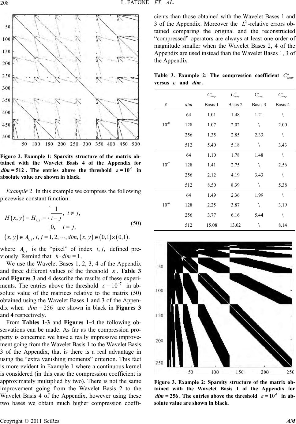

L. FATONE ET AL.

208

Figure 2. Example 1: Sparsity structure of the matrix ob-

tained with the Wavelet Basis 4 of the Appendix for

512dim =. The entries above the threshold -6

=10ε in

absolute value are shown in black.

Example 2. In this example we compress the following

piecewise constant function:



 

1,,

,==

0,= ,

,,,=1,2,,,,0,10,1 .

Hxy H

xyAijdim xy













(50)

where ,ij

is the “pixel” of index ,,ij defined pre-

viously. Remind that =1hdim.

We use the Wavelet Bases 1, 2, 3, 4 of the Appendix

and three different values of the threshold



. Table 3

and Figures 3 and 4 describe the results of these experi-

ments. The entries above the threshold 7

=10





in ab-

solute value of the matrices relative to the matrix (50)

obtained using the Wavelet Bases 1 and 3 of the Appen-

dix when = 256dim are shown in black in Figures 3

and 4 respectively.

From Tables 1-3 and Figures 1-4 the following ob-

servations can be made. As far as the compression pro-

perty is concerned we have a really impressive improve-

ment going from the Wave let Basis 1 to the Wavelet Basis

3 of the Appendix, that is there is a real advantage in

using the “extra vanishing moments” criterion. This fact

is more evident in Example 1 where a continuous kernel

is considered (in this case the compression coefficient is

approximately multiplied by two). There is not the same

improvement going from the Wavelet Basis 2 to the

Wavelet Basis 4 of the Appendix, however using these

two bases we obtain much higher compression coeffi-

cients than those obtained with the Wavelet Bases 1 and

3 of the Appendix. Moreover the 2

L-relative errors ob-

tained comparing the original and the reconstructed

“compressed” operators are always at least one order of

magnitude smaller when the Wavelet Bases 2, 4 of the

Appendix are used instead than the Wavelet Bases 1, 3 of

the Appendix.

Table 3. Example 2: The compression coefficient comp



versus ε and dim .

comp



comp



comp



comp



dim Basis 1Basis 2 Basis 3 Basis 4

64 1.01 1.48 1.21 \

10-8 128 1.07 2.02 \ 2.00

256 1.35 2.85 2.33 \

512 5.40 5.18 \ 3.43

64 1.10 1.78 1.48 \

10-7 128 1.41 2.75 \ 2.56

256 2.12 4.19 3.43 \

512 8.50 8.39 \ 5.38

64 1.49 2.36 1.99 \

10-6 128 2.25 3.87 \ 3.19

256 3.77 6.16 5.44 \

512 15.08 13.02

\ 8.14

Figure 3. Example 2: Sparsity structure of the matrix ob-

tained with the Wavelet Basis 1 of the Appendix for

256dim =. The entries above the threshold -7

=10ε in ab-

solute value are shown in black.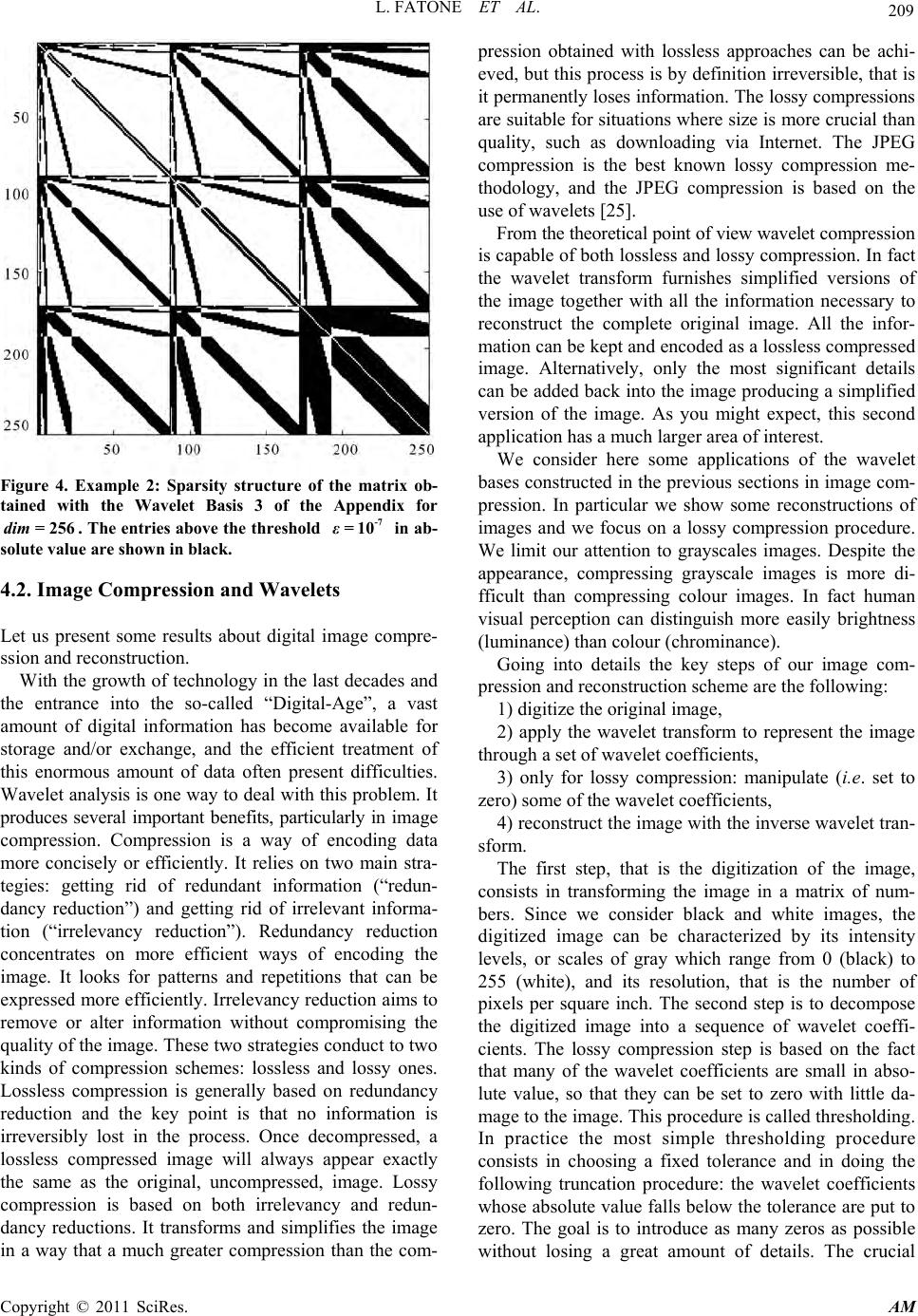

L. FATONE ET AL.

209

Figure 4. Example 2: Sparsity structure of the matrix ob-

tained with the Wavelet Basis 3 of the Appendix for

256dim=. The entries above the threshold -7

=10ε in ab-

solute value are shown in black.

4.2. Image Compression and Wavelets

Let us present some results about digital image compre-

ssion and reconstruction.

With the growth of technology in the last decades and

the entrance into the so-called “Digital-Age”, a vast

amount of digital information has become available for

storage and/or exchange, and the efficient treatment of

this enormous amount of data often present difficulties.

Wavelet analysis is one way to d eal with this problem. It

produces several important benefits, particularly in image

compression. Compression is a way of encoding data

more concisely or efficiently. It relies on two main stra-

tegies: getting rid of redundant information (“redun-

dancy reduction”) and getting rid of irrelevant informa-

tion (“irrelevancy reduction”). Redundancy reduction

concentrates on more efficient ways of encoding the

image. It looks for patterns and repetitions that can be

expressed more efficiently. Irrelevancy reduction aims to

remove or alter information without compromising the

quality of the image. These two strategies condu ct to two

kinds of compression schemes: lossless and lossy ones.

Lossless compression is generally based on redundancy

reduction and the key point is that no information is

irreversibly lost in the process. Once decompressed, a

lossless compressed image will always appear exactly

the same as the original, uncompressed, image. Lossy

compression is based on both irrelevancy and redun-

dancy reductions. It transforms and simplifies the image

in a way that a much greater compression than the com-

pression obtained with lossless approaches can be achi-

eved, but this process is by definition irreversible, th at is

it permanently loses informatio n. The lossy compressions

are suitable for situations where size is more crucial th an

quality, such as downloading via Internet. The JPEG

compression is the best known lossy compression me-

thodology, and the JPEG compression is based on the

use of wavelets [25].

From the theoret ical po int of v iew wavelet c o mpr e s s i o n

is capable of both lossless and lossy compression. In fact

the wavelet transform furnishes simplified versions of

the image together with all the information necessary to

reconstruct the complete original image. All the infor-

mation can be kept and encoded as a lossless compressed

image. Alternatively, only the most significant details

can be added back into the image producing a simplified

version of the image. As you might expect, this second

application has a much larger area of interest.

We consider here some applications of the wavelet

bases constructed in the previous sections in image com-

pression. In particular we show some reconstructions of

images and we focus on a lossy compression procedure.

We limit our attention to grayscales images. Despite the

appearance, compressing grayscale images is more di-

fficult than compressing colour images. In fact human

visual perception can distinguish more easily brightness

(luminance) than colour (chrominance).

Going into details the key steps of our image com-

pression and reconstruction scheme are the following:

1) digitize the original image,

2) apply the wavelet transform to represent the image

through a set of wavelet coefficien ts,

3) only for lossy compression: manipulate (i.e. set to

zero) some of the wavelet coefficients,

4) reconstruct the image with the inv erse wavelet tran-

sform.

The first step, that is the digitization of the image,

consists in transforming the image in a matrix of num-

bers. Since we consider black and white images, the

digitized image can be characterized by its intensity

levels, or scales of gray which range from 0 (black) to

255 (white), and its resolution, that is the number of

pixels per square inch. The second step is to decompose

the digitized image into a sequence of wavelet coeffi-

cients. The lossy compression step is based on the fact

that many of the wavelet coefficients are small in abso-

lute value, so that they can be set to zero with little da-

mage to the image. This procedure is called thresho lding.

In practice the most simple thresholding procedure

consists in choosing a fixed tolerance and in doing the

following truncation procedure: the wavelet coefficients

whose absolute value falls belo w the tolerance are put to

zero. The goal is to introduce as many zeros as possible

without losing a great amount of details. The crucial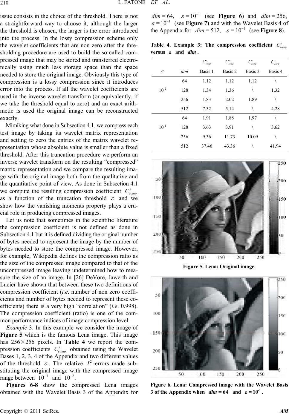

L. FATONE ET AL.

210

issue consists in the choice of the threshold. There is no t

a straightforward way to choose it, although the larger

the threshold is chosen, the larger is the error introduced

into the process. In the lossy compression scheme only

the wavelet coefficients that are non zero after the thre-

sholding procedure are used to build the so called com-

pressed image that may be stored and transferred electro-

nically using much less storage space than the space

needed to store the original image. Obviously th is type of

compression is a lossy compression since it introduces

error into the process. If all the wavelet coefficients are

used in the inverse wav elet transform (or equivalently, if

we take the threshold equal to zero) and an exact arith-

metic is used the original image can be reconstructed

exactly.

Mimiking what done in Subsection 4.1, we com press each

test image by taking its wavelet matrix representation

and setting to zero the entries of the matrix wavelet re-

presentation whose absolute value is smaller than a fixed

threshold. After this truncation procedure we perform an

inverse wavelet transform on the resulting “compressed”

matrix representation and we compare the resulting ima-

ge with the original image both from the qualitative and

the quantitative point of view. As done in Subsection 4.1

we compute the resulting compression coefficient comp



as a function of the truncation threshold



and we

show how the vanishing moments property plays a cru-

cial role in producing compressed images.

Let us note that sometimes in the scientific literature

the compression coefficient is not defined as done in

S u bsection 4.1 but it is defined d ividing the original number

of bytes needed to represent the image by the number of

bytes needed to store the compressed image. However,

for example, Wikipedia defines the compression ratio as

the size of the compressed image compared to that of the

uncompressed image leaving undetermined how to mea-

sure the size of an image. In [26] DeVore, Jawerth and

Lucier have shown that between these two definitions of

compression coefficient (i.e. number of non zero coeffi-

cients and number of bytes needed to represent these co-

efficients) there is a very high “correlation” (i.e. 0.998).

The compression coefficient (ratio) is one of the com-

mon performance indices of image compression level.

Example 3. In this example we consider the image of

Figure 5 which is the famous Lena image. This image

has 256256 pixels. In Table 4 we report the com-

pression coefficients comp



obtained using the Wavelet

Bases 1, 2, 3, 4 of the Appendix and two different values

of the threshold



. The relative 2

L-errors made sub-

stituting the original image with the compressed image

range between 3

10 and 2

10.

Figures 6-8 show the compressed Lena images

obtained with the Wavelet Basis 3 of the Appendix for

=64,dim 1

=10





(see Figure 6) and = 256,dim

=10





(see Figure 7) and with the Wavelet Basis 4 of

the Appendix fo r =512,dim 1

=10



 (see Figure 8).

Table 4. Example 3: The compression coefficient comp



versus ε and dim .

comp



comp



comp



comp



dim Basis 1Basis 2 Basis 3 Basis 4

64 1.12 1.12 1.12 \

10-2 128 1.34 1.36 \ 1.32

256 1.83 2.02 1.89 \

512 7.32 5.14 \ 4.28

64 1.91 1.88 1.97 \

10-1 128 3.63 3.91 \ 3.62

256 9.36 11.73 10.09

512 37.46 43.36

\ 41.94

Figure 5. Lena: Original image .

Figure 6. Lena: Compressed image with the Wavelet Basis

3 of the Appendix when 64dim= and -1

=10ε.

L. FATONE ET AL.

211

Figure 7. Lena: Compressed image with the Wavelet Basis

3 of the Appendix when 256dim = and -1

=10ε.

Figure 8. Lena: Compressed image with the Wavelet Basis

4 of the Appendix when 512dim = and -1

=10ε.

Example 4. We consider the image of Figure 9. In this

image are evident three different types of objects: a

shape (the black star), a number (‘2025’) and an inscri-

ption (‘black’). This image has 278268 pixels. Table 5

shows the compression coefficients comp



obtained

using the Wavelet Bases 1, 2, 3, 4 of the Appendix and

two different values of the threshold



. The relative

L-errors made substituting the original image with the

compressed image range between 3

10 and 2



Figures 10-12 show the compressed images of Figure

9 obtained for =128,dim 1

=510





 and the Wavelet

Bases 1, 2, 4 of the Appendix respectively. Figures

13-15 show the compressed images of Figure 9 obtained

for = 256,dim 1

=10



 and the Wavelet Bases 1, 2, 3

of the Appendix respectively.

The comparisons between Tables 4-5 and Figures

5-15 suggest the following observations and comments.

With respect to the compression property there is a

different behaviour of the Wavelet Bases 1, 2, 3, 4 of the

Appendix between operator compression and image

Table 5. Example 4: The compression coefficient ε

comp

versus ε and dim .

comp



comp



comp



comp



dim Basis 1Basis 2 Basis 3Basis 4

64 2.42 2.30 2.48 \

10-1 128 4.55 4.75 \ 4.23

256 11.73 13.29 12.67 \

512 38.53 46.56 \ 42.50

64 4.77 5.23 5.09 \

5 10-1 128 14.14 15.18 \ 14.38

256 52.68 56.69 53.63 \

512 208.05 226.38 \ 217.73

Figure 9. Example 4: Original image.

Figure 10. Example 4: Compressed image with the Wavelet

Basis 1 of the Appendix when 128

dim = and



-1

=5 10ε.

L. FATONE ET AL.

212

Figure 11. Example 4: Compressed image with the Wavelet

Basis 2 of the Appendix when 128

dim = and



-1

=5 10ε.

Figure 12. Example 4: Compressed image with the Wavelet

Basis 4 of the Appendix when 128

dim = and



-1

=5 10ε.

Figure 13. Example 4: Compressed image with the Wavelet

Basis 1 of the Appendix when 256

dim = and -1

=10ε.

Figure 14. Example 4: Compressed image with the Wavelet

Basis 2 of the Appendix when 256

dim = and -1

=10ε.

Figure 15. Example 4: Compressed image with the Wavelet

Basis 3 of the Appendix when 256

dim = and -1

=10ε.

compression. In fact in this last case the use of the Wave-

let Bases 1 and 3 (made of piecewise polynomial func-

tions made of polynomials of degree zero and obtained

with the two different criteria proposed in Section 2) and

the use of Wavelet Bases 2 and 4 (made of piecewise

polynomial functions made of polynomials of degree one

and obtained with the two different criteria proposed in

Section 2) furnish similar compression coefficients. This

is not really surprising since the images have a natural

discontinuity structure given by the pixels. Nevertheless

the compression coefficients obtained with the Wavelet

Basis 3 are always higher than those obtained using the

Wavelet Basis 1 and the Wavelet Bases 2 and 4 give

compression coefficients higher than those obtained with

the Wavelet Bases 1 and 3. Furthermore the use of the

Wavelet Bases 2 and 4 seems to have a regularizing effe-

ct on the images, that is the images reconstructed with

these two bases appear to have a smaller number of

L. FATONE ET AL.

213

edges and less contrast than those obtained using the Wa-

velet Bases 1 and 3.

As far as the reconstruction of the images is concerned,

we can say that very satisfactory reconstructions are ob-

tained when the dimension of the vector space generated

by the truncated wave let basis raised to the power two is

about the same than the number of pixels of the image

considered. Furthermore the relative 2

L-errors made

substituting the original image with the reconstructed

image have approximately the same order of magnitude

independently from the basis used.

Finally the following conclusions can be made. In

order to manipulate correctly operators and images it is

sufficient to construct the wavelet bases with piecewise

polynomial functions made of polynomials of very low

degree. Really for the images seems to be adequate choo-

sing piecewise polynomial functions made of polynomi-

als of degree zero. As already observed this might be due

to the way we calculate the wavelet coefficients and to

the fact that the operators and the images are represented

by piecewise constant functions. Moreover it seems to be

very promising the idea of increasing the number of va-

nishing moments keeping low the degree of the polyno-

mials used. Actually the bases that have a large number

of extra vanishing moments, that is those constructed

with the second criterion proposed in Section 2, show

better compression and reconstruction properties, and in

general work better than the wavelet bases constructed

with the first criterion proposed in Section 2.

5. References

[1] S. Mallat, “Multiresolution Approximation and Wavelets,”

Transactions of the American Mathematical Society, Vol.

315, 1989, pp. 69-88.

[2] S. Mallat, “Multifrequency Channel Decompositions of

Images and Wavelet Models,” IEEE Transactions on

Acoustics, Speech, and Signal Processing, Vol. 37, 1989,

pp. 2091-2110. doi:10.1109/29.45554

[3] Y. Meyer, “Ondelettes, Fonctions Splines et Analyses

Graduées,” Rendiconti del Seminario Matematico Uni-

versità e Politecnico di Torino, Vol. 45, 1988, pp. 1-42.

[4] Y. Meyer, “Ondelettes et Opérateurs I: Ondelettes,”

Hermann, Paris, 1990.

[5] Y. Meyer, “Ondelettes et Opérateurs II: Opérateurs de

Calderón-Zygmund,” Hermann, Paris, 1990.

[6] R. R. Coifman and Y. Meyer, “Ondelettes et Opérateurs III:

Opérateurs multilinéaires,” Hermann, Paris, 1991.

[7] I. Daubechies, “Orthonormal Bases of Compactly Sup-

ported Wavelets,” Communications on Pure and Applied

Mathematics, Vol. 41, No. 7, 1998, pp. 909-996.

doi:10.1002/cpa.3160410705

[8] I. Daubechies, “Ten Lectures on Wavelets,” SIAM, Phila-

delphia, 1992.

[9] B. K. Alpert, “Wavelets and Other Bases for Fast

Numerical Linear Algebra,” In: C. K. Chui, Ed., Wavelets:

A Tutorial in Theory and Applications, Academic Press,

New York, 1992, pp. 181-216.

[10] B. K. Alpert, “A Class of Bases in L2 for the Sparse

Representation of Integral Operators,” SIAM Journal on

Mathematical Analysis, Vol. 24, No. 1, 1993, pp. 246-262.

doi:10.1137/0524016

[11] L. Fatone, M. C. Recchioni and F. Zirilli, “New Scattering

Problems and Numerical Methods in Acoustics,” In: S. G.

Pandalai, Recent Research Developments in Acoustics,

Transworld Research Network, Kerala, Vol. 2, 2005, pp.

39-69.

[12] L. Fatone, G. Rao, M. C. Recchioni and F. Zirilli, “High

Performance Algorithms Based on a New Wavelet Ex-

pansion for Time Depende nt Acou stic Obst acle Sca ttering,”

Communications in Computational Physics, Vol. 2, No. 6,

2007, pp. 1139-1173.

[13] C. A. Micchelli and Y. Yu, “Using the Matrix Re-

finement Equation for the Construction of Wavelets on

Invariant Sets,” Applied and Computational Harmonic

Analysis, Vol. 1, No. 4, 1994, pp. 391-401.

doi:10.1006/acha.1994.1024

[14] C. A. Micchelli and Y. Yu, “Reconstruction and Decom-

position Algorithms for Biorthogonal Multi-Wavelets,”

Multidimensional Systems and Signal Processing, Vol. 8,

No. 1-2, 1997, pp. 31-69. doi:10.1023/A:1008264805830

[15] B. K. Alpert, G. Beylkin, R. R. Coifman and V. Rokhlin,

“Wavelet-Like Bases for the Fast Solution of Second-Kind

Integral Equations,” SIAM Journal on Scientific Computing,

Vol. 14, No. 1, 1993, pp.159-184. doi:10.1137/0914010

[16] L. Fatone, M. C. Recchioni and F. Zirilli, “A Numerical

Method for Time Dependent Acoustic Scattering Problems

Involving Smart Obstacles and Incoming Waves of Small

Wavelengths,” In: B. Nilsson and L. Fishman, Eds.,

Mathematical Modeling of Wave Phenomena, AIP Con-

ference Proceedings, Khanty-Mansiysk, Vol. 834, 17-22

July 2006, pp. 108-121.

[17] W. Rudin, “Real and Complex Analysis,” Mc Graw Hill

Inc., New York, 1966.

[18] J. Stoer and R. Bulirsch, “Introduction to Numerical

Analysis,” Springer-Verlag, New York, 2002.

[19] G. Beylkin, R. R. Coifman and V. Rokhlin, “Fast Wavelet

Transforms and Numerical Algorithms I,” Communications

on Pure and Applied Mathematics, Vol. 44, No. 2, 1991,

pp. 141-183. doi:10.1002/cpa.3160440202

[20] W. Sweldens and R. Piessens, “Quadrature Formulae and

Asymptotic Error Expansions for Wavelet Appr oximations

of Smooth Functions,” SIAM Journal on Numerical

Analysis, Vol. 31, No. 4, 1994, pp. 1240-1264.

doi:10.1137/0731065

[21] D. Huybrechs and S. Vandewalle, “Composite Quadrature

Formulae for the Approximations of Wavelet Coeffi-

cients of Piecewise Smooth and Singular Functions,”

Journal of Computational and Applied Mathematics, Vol.

180, No. 1, 2005, pp. 119-135.

doi:10.1016/j.cam.2004.10.005

L. FATONE ET AL.

214

[22] W. Gautschi, L. Gori and F. Pitolli, “Gauss Quadrature

Rules for Refinable Weight Functions,” Applied and

Computational Harmonic Analysis, Vol. 8, No. 3, 2000,

pp. 249-257. doi:10.1006/acha.1999.0306

[23] A. Barinka, T. Barsch, S. Dahlke and M. Konik, “Some

Remarks on Quadrature Formulas for Refinable Functions

and Wavelets,” ZAMM Journal of Applied Mathematics

and Mechanics, Vol. 81, No. 12, 2001, pp. 839-855.

doi:10.1002/1521-4001(200112)81:12<839::AID-ZAMM

839>3.0.CO;2-F

[24] F. Keinert, “Biorthogonal Wavelets for Fast Matrix Com-

putations,” Applied and Computational Harmonic Analy-

sis, Vol. 1, No. 2, 1994, pp. 147-156.

doi:10.1006/acha.1994.1002

[25] D. S. Taubman and M. W. Marcellin, “JPEG2000: Image

Compression Fundamentals, Standards and Practice,” Kluwer

Academic Publishers, Boston, 2002.

[26] R. A. DeVore, B. D. Jawerth and B. J. Lucier, “Image

Compression through Wavelet Transform Coding,” IEEE

Transactions on Information Theory, Vol. 38, No. 2, 1992,

pp. 719-746. doi:10.1109/18.119733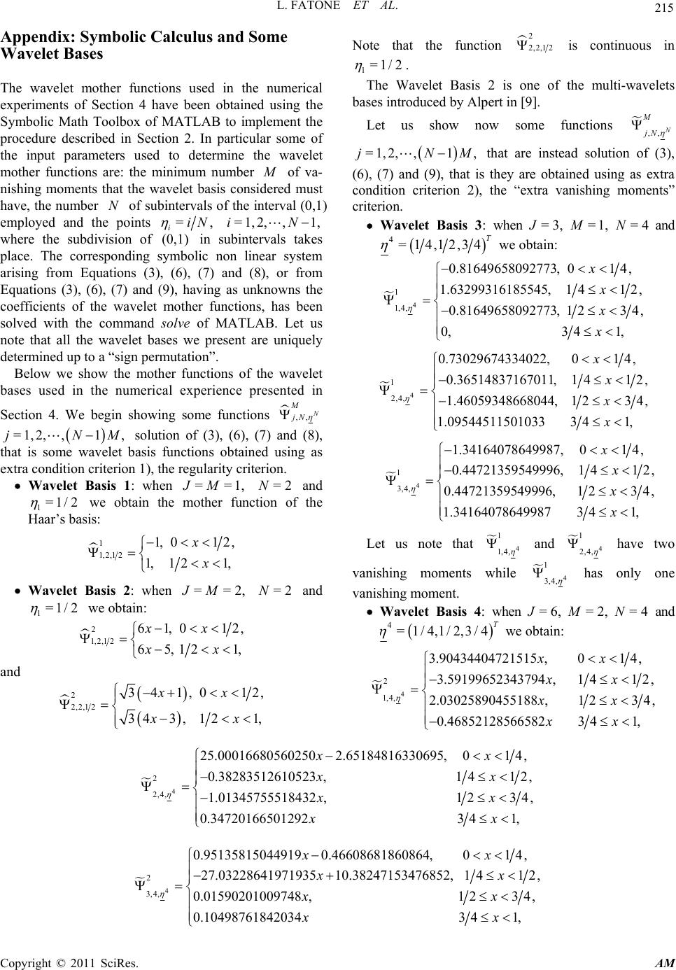

L. FATONE ET AL.

215

Appendix: Symbolic Calculus and Some

Wavelet Bases

The wavelet mother functions used in the numerical

experiments of Section 4 have been obtained using the

Symbolic Math Toolbox of MATLAB to implement the

procedure described in Section 2. In particular some of

the input parameters used to determine the wavelet

mother functions are: the minimum number

of va-

nishing moments that the wavelet basis considered must

have, the number N of subintervals of the interval (0,1)

employed and the points =,

iiN



=1,2,,1,iN





where the subdivision of (0,1) in subintervals takes

place. The corresponding symbolic non linear system

arising from Equations (3), (6), (7) and (8), or from

Equations (3), (6), (7) and (9), having as unknowns the

coefficients of the wavelet mother functions, has been

solved with the command solve of MATLAB. Let us

note that all the wavelet bases we present are uniquely

determined up to a “sign permutation”.

Below we show the mother functions of the wavelet

bases used in the numerical experience presented in

Section 4. We begin showing some functions











=1,2,,1,jNM solution of (3), (6), (7) and (8),

that is some wavelet basis functions obtained using as

extra condition criterion 1), the regularity criterion.

 Wavelet Basis 1: when ==1,JM =2N and

1=1/ 2



we obtain the mother function of the

Haar’s basis:



1,2,1 21,012 ,

1,121,











 Wavelet Basis 2: when ==2,JM =2N and

1=1/ 2



we obtain:



1,2,1 261,0 12,

65,12 1,











and





2,2,1 2341,012,

343, 121,

 











Note that the function



2,2,1 2

 is continuous in

1=1/2



The Wavelet Basis 2 is one of the multi-wavelets

bases introduced by Alpert in [9].

Let us show now some functions











=1,2,,1,jNM that are instead solution of (3),

(6), (7) and (9), that is they are obtained using as extra

condition criterion 2), the “extra vanishing moments”

criterion.

 Wavelet Basis 3: when = 3,

=1,M =4N and



4=14,12,34



we obtain:



1,4,

0.81649658092773,01 4,

1.63299316185545,141 2,

0.81649658092773,1 234,

0,3 41,























2,4,

0.73029674334022,01 4,

0.36514837167011,1412,

1.46059348668044,1 234,

1.095445115010333 41,























3,4,

1.34164078649987,01 4,

0.44721359549996,141 2,

0.44721359549996,1 234,

1.341640786499873 41,





















Let us note that



1,4,



 and



2,4,



 have two

vanishing moments while



3,4,



 has only one

vanishing moment.

 Wavelet Basis 4: when = 6,

=2,M =4N and



4= 1/4,1/2,3/4



we obtain:



1,4,

3.90434404721515,01 4,

3.59199652343794,141 2,

2.03025890455188,1 234,

0.468521285665823 41,























2,4,

25.000166805602502.65184816330695,01 4,

0.38283512610523,141 2,

1.01345755518432,1 234,

0.347201665012923 41,























3,4,

0.951358150449190.46608681860864,01 4,

27.0322864197193510.38247153476852,141 2,

0.01590201009748,1 234,

0.104987618420343 41,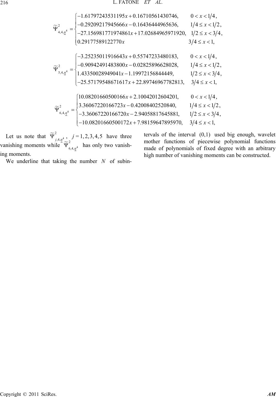







 













L. FATONE ET AL.

216



4,4,

1.617972435311950.16710561430746,01 4,

0.292092179456660.16436444965636,1412,

27.15698177197486117.02684965971920,1 234,

0.291775891227703 41,



 



 





 









5,4 ,

3.252350119166430.55747233480183,01 4,

0.909424914838000.02825896628028,141 2,

1.433500289490411.19972156844449,1 234,

25.5717954867161722.89746967782813,3 41,



 













 





6,4,

10.082016605001662.10042012604201,01 4,

3.360672201667230.42008402520840,141 2,

3.360672201667202.94058817645881,1 234,

10.082016605001727.98159647895970,3 41,

















 



Let us note that



,4,



, = 1,2,3,4,5j have three

vanishing moments while



6,4,



 has only two vanish-

ing moments.

We underline that taking the number N of subin-

tervals of the interval (0,1) used big enough, wavelet

mother functions of piecewise polynomial functions

made of polynomials of fixed degree with an arbitrary

high number of vanishing moments can be constructed.