 Energy and Power Engineering, 2013, 5, 1126-1133 doi:10.4236/epe.2013.54B215 Published Online July 2013 (http://www.scirp.org/journal/epe) The Use of LMS and RLS Adaptive Algorithms for an Adaptive Co ntrol Method o f Active Pow e r Filter Radek Martinek1, Jan Zidek1, Petr Bilik1, Ja kub M anas 1, Jiri Koziorek1, Zhaosheng Teng2, He Wen2 1Faculty of Electrical Engineering and Computer Science, VSB – Technical University of Ostrava, Czech Republic 2College of Electrical and Information Engineering, Hunan University, Changsha, Hunan Province, China Email: {radek.martinek, jan.zidek, petr.bilik, jakub.manas, jiri.koziorek}@vsb.cz, tengzs@126.com, he_wen@hnu.edu.cn Received March, 2013 ABSTRACT This paper deals with the adaptive control mechanism management meant for shunt active power filters (SAPF). Sys- tems driven this way are designed to improve the quality of electric power (power quality) in industrial networks. The authors have focused on the implementation of two basic representatives of adaptive algorithms, first, the algorithm with a stochastic LMS (least mean square) gradient adaptation and then an algorithm with recursive RLS (recursive least square) optimal adaptation. The system examined by the authors can be used for non-linear loads for appliances with rapid fluctuations of the reactive and active power consumption. The proposed system adaptively reduces distor- tion, falls (dip) and changes in a sup p ly voltage (flicker). Real signals for measurement were obtained at a sophisticated, three-phase experimental workplace. The results of executed experiments indicate that, with use of the certain adaptive algorithms, the examined AHC system shows very good dynamics, resulting in a much faster transition during the AHC connection-disconnection or during a change in harmonic load on the network. The actual experiments are evaluated from several points of view, mainly according to a time convergence (convergence time) and mistakes in a stable state error (steady state error) of the investigated adaptive algorithms and finally as a total harmonic distortion (THD). The article presents a comparison of the most frequ ently used adaptiv e algorithms. Keywords: Active Power Filters; Total Harmonic Distortion; Least Mean Square; Adap tive Filtering; Recursive Least Square 1. Introduction Currently, the active harmonic compensation AHC [1], which is intended to compensate the harmonic flow gen- erated by the powerful electronics, is being used more and more often in the industrial applications [2]. Modern industrial corporations usually have numerous types of electrical equipment and the load [2] which can be di- vided into the linear load [24] (regenerative power unit, active loads, standing on alternating current) and non-linear loads [23] (variable speed drives, arc units, etc.). The authors of this article have primarily focused on adaptive filters [20] from the viewpoint of ad aptive algo- rithms utilized [13] in order to improve efficiency of the Active Power Filters - APF [23]. This article concen- trates on the adaptive control method - ACM [7] de- signed for the APF, especially from perspective of the examining the performance data of adaptive algorithms used. The authors do not deeper examine their own APF project as this topic is very broad and it has been covered in a number of vari ous pu bl i cat ions s uc h as: [ 4, 1 4, 2 2]. In the framework of the experiment, the investigated algorithms least mean squares – the LMS [5] based adap- tive FIR filters [5] and recursive least squares – the RLS [5] based adaptive FIR filters [5 ] were tested on real sig- nals. Real data were obtained at the earlier mentioned three-phase experimental workplace, see Picture 3. 2. The Situation in 2013 At present, we can see notable development in the indu s- trial APF supply networks [2]. The role of active com- pensation is increase of its importance alongside with the passive filters [22], which are traditionally used to im- prove the quality of a power supply. However these tra- ditional approaches in the form of a passive compensa- tion have, from the perspective of modern power net- works, certain disadvantages [22]. We are talking espe- cially about situations where the proposed filter has to operate in an unfamiliar environment, where preliminary identification is difficult. Here, it is hard to set the filter parameters [9] to solve the given task in th e best possible way. Another case is where there is an environment with a variable (where there are various, unspecified loads Copyright © 2013 SciRes. EPE 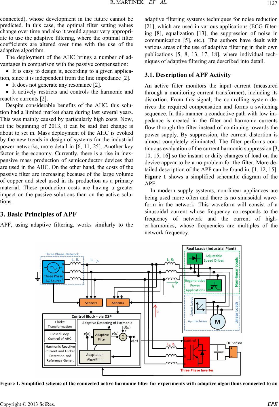 R. MARTINEK ET AL. 1127 connected), whose development in the future cannot be predicted. In this case, the optimal filter setting values change over time and also it would appear very appropri- ate to use the adaptive filtering, where the optimal filter coefficients are altered over time with the use of the adaptive algorithm. The deployment of the AHC brings a number of ad- vantages in comparison with the passive compensation: It is easy to design it, according to a given applica- tion, since it is independ ent from the line impedance [2]. It does not generate any resonance [2]. It actively restricts and controls the harmonic and reactive currents [2]. Despite considerable benefits of the AHC, this solu- tion had a limited market share during last several years. This was mainly caused by particularly high costs. Now, at the beginning of 2013, it can be said that change is about to set in. Mass deployment of the AHC is evoked by the new trends in design of systems for the industrial power networks, more detail in [6, 11, 25]. Another key factor is the economy. Currently, there is a rise in inex- pensive mass production of semiconductor devices that are used in the AHC. On the other hand, the costs of the passive filter are increasing because of the large volume of copper and steel used in its production as a primary material. These production costs are having a greater impact on the passive solutions than on the active solu- tions. 3. Basic Principles of APF APF, using adaptive filtering, works similarly to the adaptive filtering systems techniques for noise reduction [21], which are used in various applications (ECG filter- ing [8], equalization [13], the suppression of noise in communication [5], etc.). The authors have dealt with various areas of the use of adaptive filtering in their own publications [5, 8, 13, 17, 18], where individual tech- niques of adaptive filtering are de scribed into detail. 3.1. Description of APF Activity An active filter monitors the input current (measured through a monitoring current transformer), including its distortion. From this signal, the controlling system de- rives the required compensation and forms a switching sequence. In this manner a conduc tive path with low im- pedance is created in the filter and harmonic currents flow through the filter instead of continuing towards the power supply. By suppression, the current distortion is almost completely eliminated. The filter performs con- tinuous evaluation of the current harmonic suppression [3, 10, 15, 16] so the instant or daily changes of load on the device appear to be a no problem for the filter. More de- tailed description of the APF can be found in, [1, 12, 15]. Figure 1 shows a simplified schematic diagram of the APF. In modern supply systems, non-linear appliances are being used more often and there is no sinusoidal wave- form in the network. This waveform will consist of a sinusoidal current whose frequency corresponds to the frequency of network and the current of high- er harmonics, whose frequencies are multiples of the network frequency. Figure 1. Simplified scheme of the connected active harmonic filter for experiments with adaptive algorithms connected to an Copyright © 2013 SciRes. EPE 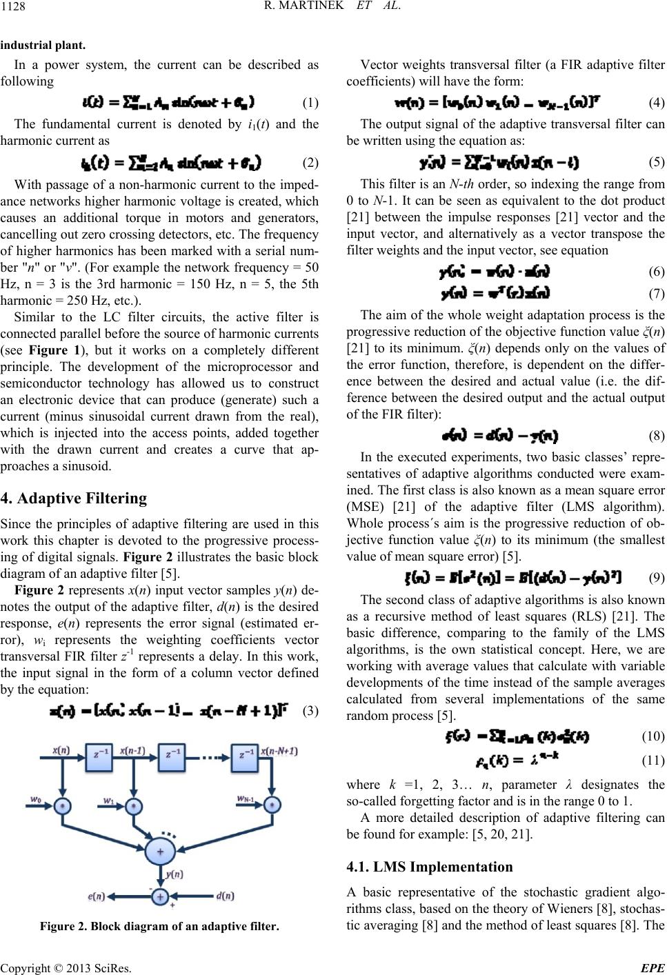 R. MARTINEK ET AL. 1128 i ndustrial plant. In a power system, the current can be described as following (1) The fundamental current is denoted by i1(t) and the harmonic current as (2) With passage of a non-harmonic current to the imped- ance networks higher harmonic voltage is created, which causes an additional torque in motors and generators, cancelling out zero crossing detectors, etc. Th e frequency of higher harmonics has been marked with a serial num- ber "n" or "v". (For example the network frequency = 50 Hz, n = 3 is the 3rd harmonic = 150 Hz, n = 5, the 5th harmonic = 250 Hz, etc.). Similar to the LC filter circuits, the active filter is connected parallel before the source of harmonic currents (see Figure 1), but it works on a completely different principle. The development of the microprocessor and semiconductor technology has allowed us to construct an electronic device that can produce (generate) such a current (minus sinusoidal current drawn from the real), which is injected into the access points, added together with the drawn current and creates a curve that ap- proaches a sinusoid. 4. Adaptive Filtering Since the principles of adaptive filtering are used in this work this chapter is devoted to the progressive process- ing of digital signals. Figure 2 illustrates the basic block diagram of an adaptive filter [5]. Figure 2 represents x(n) input vector samples y(n) de- notes the output of the adaptive filter, d(n) is the desired response, e(n) represents the error signal (estimated er- ror), wi represents the weighting coefficients vector transversal FIR filter z-1 represents a delay. In this work, the input signal in the form of a column vector defined by the equation: (3) Figure 2. Block diagram of an adaptive filter. Vector weights transversal filter (a FIR adaptive filter coefficients) will have the form: (4) The output signal of the adaptive transversal filter can be written using the equation as: (5) This filter is an N-th order, so indexing the range from 0 to N-1. It can be seen as equivalent to the dot product [21] between the impulse responses [21] vector and the input vector, and alternatively as a vector transpose the filter weights and the input vector, see eq uation (6) (7) The aim of the whole weight adaptation process is the progressive reduction of the objective function value ξ(n) [21] to its minimum. ξ(n) depends only on the values of the error function, therefore, is dependent on the differ- ence between the desired and actual value (i.e. the dif- ference between the desired output and the actual output of the FIR filter): (8) In the executed experiments, two basic classes’ repre- sentatives of adaptive algorithms conducted were exam- ined. The first class is also known as a mean square error (MSE) [21] of the adaptive filter (LMS algorithm). Whole process´s aim is the progressive reduction of ob- jective function value ξ(n) to its minimum (the smallest value of mean square error) [5]. (9) The sec ond class of adap tive algorithms is also known as a recursive method of least squares (RLS) [21]. The basic difference, comparing to the family of the LMS algorithms, is the own statistical concept. Here, we are working with average values that calculate with variable developments of the time instead of the sample averages calculated from several implementations of the same random process [5]. (10) (11) where k =1, 2, 3… n, parameter λ designates the so-called forgetting factor and is in the range 0 to 1. A more detailed description of adaptive filtering can be found for example: [5, 20, 21]. 4.1. LMS Implementation A basic representative of the stochastic gradient algo- rithms class, based on the theory of Wieners [8], stochas- tic averaging [8] and the method of least squares [8]. Th e Copyright © 2013 SciRes. EPE  R. MARTINEK ET AL. 1129 custom LMS algorithm derivation is generally known and described in many technical publications, such as: [5, 8, 21]. So in this article, there is only a simple mathe- matical description of the respective algorithm imple- mentation. Each items of the LMS algorithm requires three dis- tinct steps in this order: 1) The output of the FIR filter y(n) is calculated using an equation 5 or 6 and 7. 2) Value of the estimated error is calculated using equation 5. 3) FIR weight vector is updated in preparation for the next iteration of the equation [15]: (12) The parameter μ is referred as a step size. It is a small positive constant which influences the properties of the algorithm adaptation (filter stability, convergence rate, etc.). 4.2. RLS Implementation It's a basic representative of the recursive algorithms class based on the theory of Kalmans filtering [8], time averaging [8] and the method of least squares, see [8]. The basic difference comparing to the LMS algorithms family lies in the respective statistical concepts. We are working with average values calculated from the time developments, instead of the sample averages of several implementations from the same random process. The structure of the filter remains the same compared to the LMS algorithm, only the adaptive process is different because of the averages use. A detailed description and derivation of the RLS algorithm can be found in [8, 20, 21]. If we want to implement the RLS algorithm it must be carried out along the following steps in this order: 1) Filter output is calculated using the weights of the filter from the previous iteration and the current input vector: (13) 2) Medium-range vector gain is calculated using the equation: (14) (15) 3) The value of the estimated error is calculated ac- cording to the equation: (16) 4) The vector filter weights are u pdated using equ ation 16 and the vector gain is calculated in equation 15: (17) 5) The inverse matrix is calculated using the fo llowing equation: (18) 5. Experimental Workplace To real voltages and currents generation three-phase ex- perimental workplace was used with three-phase pro- grammable source HP 6834B connected as the inputs. To voltages and currents acquisition the IED (Intelli- gent Electronic Device) was built connected to the out- puts on the workplace Linear and non-linear loads were connected to work- place. Programmable source HP6834B can generate sine waveforms with maximum amplitude 300V/5A per phase with 100th harmonics. Source was connected remotely to IED (GPIB interface) for automation testing. The IED can measure up to three voltages (directly) and three currents (directly or using current clamps). For voltage and current measurement precise modules (un- certainty ±0,1%) is used with an t aliasing filters [25]. All inputs were calibrated with NI 9925 modules. Sample rate was set to 30 kS/Channel. In the IED the application was developed for PQ (Power Quality) parameters anal- ysis. The application evaluates harmonics, interharmon- ics and higher frequency components (complies with IEC 61000-4-7 standard), flicker (IEC 61000-4-15), voltage phenomena (IEC 61000-4-30) and the voltage character- istics (EN 50160). Th e app licatio n can stream raw d ata to TDMS files for offline post-processing. Figure 3. Three-phase experimental workplace. Copyright © 2013 SciRes. EPE  R. MARTINEK ET AL. 1130 An application created in IED (Pictures.5, 6) utilizes the concept of a virtual instrumentation [19], therefore there is no need for more time and resource expandable to meet future requirements for the development of adap- tive filter algorithms. 6. Results of the Experiments Carried Out In Figure 7, there is a depicted reference waveform cur- rent to the linear load. For each phase the THD [7] dis- tortion is less than 0.2%. The length of the time window of 0.1 s for all the charts is selected for the optimal dis- play of waveform. THD is a quantity that defines the distortion sin e wave. It is defined as a ratio of the all harmonic components Figure 4. Connec ted inputs and outputs of the experimental workplace without a connected load. Figure 5. Developed application graphical interface. (Waveforms). total power to the fundamental harmonic performance The lower the THD is, the more constant is the signal. THD is a way of assessing the extent of distortion. THD calculation is based on decomposition of a periodic sig- nal to harmonic components using Fourier series in the amplitude-phase entry. In Figure 8, strongly distorted waveform caused by nonlinear loads. THD distortion is for phase L1 88.1%, L2 98, 2% an d L 3 92.3%. In Figure 9, the resulting current waveform is calcu- lated using the RLS adaptive filter algorithm. THD dis- tortion is diminished for phase L1 88.1% to 5.43%, L2 98.2% to 6.43% and L3 92.3% to 4.78%.THD for the reconstructed current waveform now meets the THD limits set according to the EN 61000-3-2 standard. In Figure 10 is the output current waveform calculated using the LMS adaptive filter algorithm. THD distortion is diminished for phase L1 88.1% to 13.54%, L2 98.2% to 16.86% and 92.3% to L3 14.32%. Figure 6. Developed application graphical interface (Re- sult). Figure 7. Reference current waveform to a linear load. Copyright © 2013 SciRes. EPE 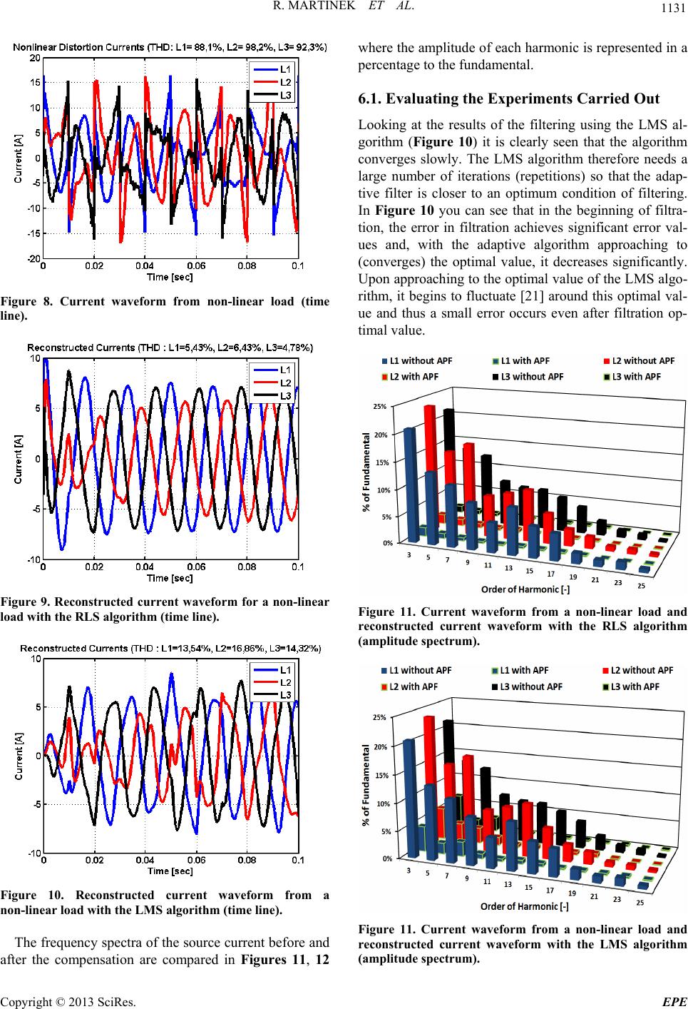 R. MARTINEK ET AL. 1131 Figure 8. Current waveform from non-linear load (time line). Figure 9. Reconstructed current waveform for a non-linear load with the RLS algorithm (time line). Figure 10. Reconstructed current waveform from a non-linear load with the LMS algorithm (time line). The frequency spectra of the source current before and after the compensation are compared in Figures 11, 12 where the amplitude of each harmonic is represented in a percentage to the fundamental. 6.1. Evaluating the Experiments Carried Out Looking at the results of the filtering using the LMS al- gorithm (Figure 10) it is clearly seen that the algorithm converges slowly. The LMS algorithm therefore needs a large number of iterations (repetitions) so that the adap- tive filter is closer to an optimum condition of filtering. In Figure 10 you can see that in the beginning of filtra- tion, the error in filtration achieves significant error val- ues and, with the adaptive algorithm approaching to (converges) the optimal value, it decreases significantly. Upon approaching to the optimal value of the LMS algo- rithm, it begins to fluctuate [21] around this optimal val- ue and thus a small error occurs even after filtration op- timal value. Figure 11. Current waveform from a non-linear load and reconstructed current waveform with the RLS algorithm (amplitude spectrum). Figure 11. Current waveform from a non-linear load and reconstructed current waveform with the LMS algorithm (amplitude spectrum). Copyright © 2013 SciRes. EPE 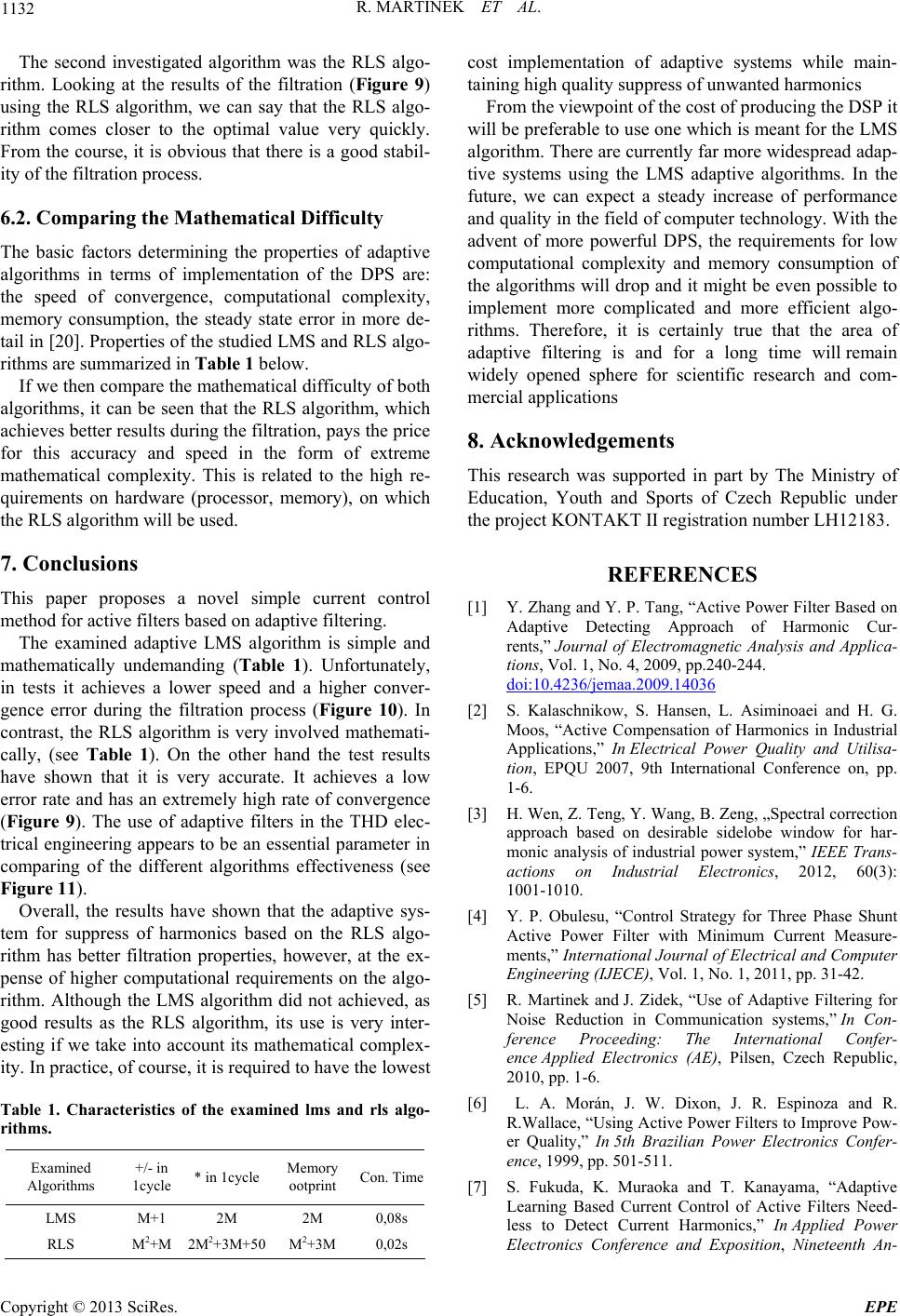 R. MARTINEK ET AL. 1132 The second investigated algorithm was the RLS algo- rithm. Looking at the results of the filtration (Figure 9) using the RLS algorithm, we can say that the RLS algo- rithm comes closer to the optimal value very quickly. From the course, it is obvious that there is a good stabil- ity of the filtration process. 6.2. Comparing the Mathematical Difficulty The basic factors determining the properties of adaptive algorithms in terms of implementation of the DPS are: the speed of convergence, computational complexity, memory consumption, the steady state error in more de- tail in [20]. Properties of the studied LMS and RLS algo- rithms are summarized in Table 1 below. If we then compare the mathematical difficulty of both algorithms, it can be seen that the RLS algorithm, which achieves better results during th e filtration, pays the price for this accuracy and speed in the form of extreme mathematical complexity. This is related to the high re- quirements on hardware (processor, memory), on which the RLS algorithm will be used. 7. Conclusions This paper proposes a novel simple current control method f o r act ive filter s ba s ed on adaptive filtering. The examined adaptive LMS algorithm is simple and mathematically undemanding (Table 1). Unfortunately, in tests it achieves a lower speed and a higher conver- gence error during the filtration process (Figure 10). In contrast, the RLS algorithm is very involved mathemati- cally, (see Table 1). On the other hand the test results have shown that it is very accurate. It achieves a low error rate and has an extremely high rate of convergence (Figure 9). The use of adaptive filters in the THD elec- trical engineering appears to be an essential parameter in comparing of the different algorithms effectiveness (see Figure 11). Overall, the results have shown that the adaptive sys- tem for suppress of harmonics based on the RLS algo- rithm has better filtration properties, however, at the ex- pense of higher computational requirements on the algo- rithm. Although the LMS algorithm did not achieved, as good results as the RLS algorithm, its use is very inter- esting if we take into account its mathematical complex- ity. In practice, of course, it is required to have the lowest Table 1. Characteristics of the examined lms and rls algo- rithms. Examined Algorithms +/- in 1cycle * in 1cycle Memory ootprint Con. Time LMS M+1 2M 2M 0,08s RLS M2+M 2M2+3M+50 M2+3M 0,02s cost implementation of adaptive systems while main- taining high quality suppress of unwanted harmonics From the viewpoint of the cost of producing the DSP it will be preferable to use on e which is meant for the LMS algorithm. There are currently far more widespread adap- tive systems using the LMS adaptive algorithms. In the future, we can expect a steady increase of performance and quality in the field of computer technolog y. With the advent of more powerful DPS, the requirements for low computational complexity and memory consumption of the algorithms will drop and it might b e even possible to implement more complicated and more efficient algo- rithms. Therefore, it is certainly true that the area of adaptive filtering is and for a long time will remain widely opened sphere for scientific research and com- mercial applications 8. Acknowledgements This research was supported in part by The Ministry of Education, Youth and Sports of Czech Republic under the project KONTAKT II registration number LH12183. REFERENCES [1] Y. Zhang and Y. P. Tang, “Active Power Filter Based on Adaptive Detecting Approach of Harmonic Cur- rents,” Journal of Electromagnetic Analysis and Applica- tions, Vol. 1, No. 4, 2009, pp.240-244. doi:10.4236/jemaa.2009.14036 [2] S. Kalaschnikow, S. Hansen, L. Asiminoaei and H. G. Moos, “Active Compensation of Harmonics in Industrial Applications,” In Electrical Power Quality and Utilisa- tion, EPQU 2007, 9th International Conference on, pp. 1-6. [3] H. Wen, Z. Te ng, Y. Wang, B. Zeng, „Spectral correction approach based on desirable sidelobe window for har- monic analysis of industrial power system,” IEEE Trans- actions on Industrial Electronics, 2012, 60(3): 1001-1010. [4] Y. P. Obulesu, “Control Strategy for Three Phase Shunt Active Power Filter with Minimum Current Measure- ments,” International Journal of Electrical and Computer Engineering (IJECE), Vol. 1, No. 1, 2011, pp. 31-42. [5] R. Martinek and J. Zidek, “Use of Adaptive Filtering for Noise Reduction in Communication systems,” In Con- ference Proceeding: The International Confer- ence Applied Electronics (AE), Pilsen, Czech Republic, 2010, pp. 1-6. [6] L. A. Morán, J. W. Dixon, J. R. Espinoza and R. R.Wallace, “Using Active Power Filters to Improve Pow- er Quality,” In 5th Brazilian Power Electronics Confer- ence, 1999, pp. 501-511. [7] S. Fukuda, K. Muraoka and T. Kanayama, “Adaptive Learning Based Current Control of Active Filters Need- less to Detect Current Harmonics,” In Applied Power Electronics Conference and Exposition, Nineteenth An- Copyright © 2013 SciRes. EPE  R. MARTINEK ET AL. Copyright © 2013 SciRes. EPE 1133 nual IEEE, Vol. 1, 2004, pp. 210-216. doi:10.1109/APEC.2004.1295812 [8] R. Martinek and J. Zidek, “A System for Improving the Diagnostic Quality of Fetal Electrocardiogram,” In Journal: Przeglad Elektrotchniczny (Electrical Re- view), Warszawa, Poland, May 2012, pp. 164-173. [9] B. M. Han, B. Y. Bae and S. J. Ovaska, “Reference Sig- nal Generator for Active Power Filters Using Improved Adaptive Predictive Filter,” Industrial Electronics, IEEE Transactions on, Vol. 52, No. 2, 2005, pp. 576-584. doi:10.1109/TIE.2005.844222 [10] H. Wen, Z. Teng, Y. Wang, B. Zeng, X. Hu, “Simple interpolated FFT algorithm based on minimize sidelobe windows for power-harmonic analysis,” IEEE Transac- tions on Power Electronics, 2011, 26(9):2570-2579. [11] A. Luo, Z. Shuai, W. Zhu, R. Fan and C. Tu, “Develop- ment of Hybrid Active Power Filter Based on the Adap- tive Fuzzy Dividing Frequency-control Method,” Power Delivery, IEEE Transactions on, Vol. 24, No. 1, 2009, pp.424-432. doi:10.1109/TPWRD.2008.2005877 [12] J. Zhang and K. Liu, “Harmonic Detection for Three-phase Circuit Based on the Improved Analog LMS Algorithm,”In Electrical Machines and Systems, ICEMS 2008, International Conference on, 2008, pp. 3978-3982 [13] R. Martinek and J. Zidek, “The Real Implementation of NLMS Channel Equalizer into the System of Software Defined Radio,” In Journal: Advances in Electrical and Electronic Engineering, Vol. 10, No. 5, 2012, pp. 330-336. [14] M. Cirrincione, M. Pucci, G. Vitale and A. Miraoui, “Current Harmonic Compensation by a Single-phase Shunt Active Power Filter Controlled by Adaptive Neural Filtering,” Industrial Electronics, IEEE Transactions on, Vol. 56, No. 8, 2009, pp. 3128-3143. doi:10.1109/TIE.2009.2022070 [15] R. R. Pereira, C. H. da Silva, G. F. C. Veloso, L. E. B. da Silva and G. L. Torres, “A New Strategy to Step-size Control of Adaptive Filters in the Harmonic Detection for Shunt Active Power Filter,” In Industry Applications So- ciety Annual Meeting, 2009, pp. 1-5. [16] H. Wen, Z. Teng, S. Guo. “Triangular self-convolution window with desirable sidelobe behaviors for harmonic analysis of power system,” IEEE Transactions on In- strumentation and Measurement, 2010, 59 (3): 543-552. [17] M. McGranaghan, “Active Filter Design and Specifica- tion for Control of Harmonics in Industrial and Commer- cial Facilities,” Electrotek Concepts Inc. [18] J. G. Avalos, J. C. Sanchez and J. Velazquez, “Applica- tions of Adaptive Filtering,” 2011. [19] R. Martinek, M. Al-Wohaishi and J. Zidek, “Software Based Flexible Measuring Systems for Analysis of Digi- tally Modulated Systems,” In Conference Proceedings: The 9th Roedunet International Conference, RoEduNet, Sibiu, Romania, 2010, pp. 397-402. [20] Haykin and Simon. “Adaptive Filter Theory” 4th. New Jersey: Prentice Hall, 2001. [21] B. Farhang-Boroujrny, “Adaptive Filters: Theory and Applications,” New York: John Wiley and Sons, 1999. [22] M. Rashid, “Power Electronics Handbook, Hardbound,” Published: December 2010, Butterworth Heinemann, p.1362. [23] Z. Salam, “Hybrid Active Power Filter,” LAP Lambert Academic Publishing, 2009, p.184. [24] J. B. Dixit, “Amit Yadav, Electrical Power Quality, First,” 2010, p. 172. [25] V. Kus and B. Skala, “Aliasing Effect in Power Electron- ics,” In Conference Proceedings: Applied Electronics AE 2011, Pilsen, CzechRepublic, 2010, pp. 213-216.
|