 Energy and Power Engineering, 2013, 5, 970-974 doi:10.4236/epe.2013.54B186 Published Online July 2013 (http://www.scirp.org/journal/epe) Lagrangian Relaxation-Based Unit Commitment Considering Fast Response Reserve Constraints* C. S. Chuang, G. W. Chang Department of Electrical Engineering, National Chung Cheng University Email: wchang@ee.ccu.edu.tw Received September, 2012 ABSTRACT Unit commitment (UC) is to determine the optimal unit status and generation level during each time interval of the scheduled period. The purpose of UC is to minimize the total generation cost while satisfying system demand, reserve requirements, and unit constraints. Among the UC constraints, an adequate provision of reserve is important to ensure the security of power system and the fast-response reserve is essential to bring system frequency back to acceptable level following the loss of an online unit within a few seconds. In this paper, the au thors present and solve a UC prob- lem including the frequency-based reserve constraints to determine the optimal FRR requirements and unit MW sched- ules. The UC problem is solved by using Lagrangian Relaxation-based approach and compared with the actual system schedules. It is observed that favorable reserve and unit MW schedules are obtained by the proposed method while the system security is maintained. Keywords: Unit Commitment; Fast Response Reserve; Frequency-based Reserve Constraints; Lagrangian Relaxation 1. Introduction The unit commitment (UC) problem is to optimize hour- ly schedules of unit operation and minimize system op- erating costs for a given time interval. The constraints that the schedules must meet include system demand, reserve requirements, and unit constraints. Among the system constraints, the reserve is a crucial requirement for maintaining system frequency within the normal lim- its without any load shedding when the system experi- ences a contingency. Especially for an isolated power system, the system frequency is sensitive in responding to the load variation. Therefore, it is extremely impor tant to schedule sufficient fast-response reserve (FRR) capac- ity to maintain the system security. The response time of FRR is usually the order of seconds to arrest the initial fall in frequency following the loss of any online genera- tion unit. Therefore, the criterion of determining the FRR is difficult, since it varies from system to system. In [1] and [2], the load-frequency sensitivity index (LFSI) was used to assess the frequency drop following the loss of the largest online unit. However, this method still had to recalculate the reserve levels until the frequency con- straint was met by an iterative procedure. In this paper, the frequency-based reserve constraints are considered in the UC problem. The LFSI and unit MW schedules are determined simultaneously. Then, the required FRR at each time step without violating the minimum system frequency is obtained. The UC problem including fre- quency reserve-based constraint is described and the problem is solved by using Lagrangian Relaxation-based approach. Simulation results and numerical experiences compared with the actual system are the reported. 2. Problem Formulation The following gives the addressed UC problem formula- tion. More details can be found in [3] and [4]. 2.1. Objective Function The objective function is to minimize the operation cost, the cost of power purchase, and the compensation cost of violating the number of limit associated with independent power pr od u cers’ (IPP) uni t startup a nd shu tdown. , ,, ,,, ,,,,,, 1 ,,,, , ()()( ) ()()() ()() Ti c pp tt t iii uii di tTiN N tt t i cicijuijcijdij tTiN j tt ip iip iph iyz iss imi ph,i tTiN iN FfpyCzC cf pyCCzCC pup CTNC , (1) where fi and cfi are the fuel cost functions for the thermal and combined-cycle un its; Cu,i, Cd,i, CCu,i,j, and CCd,i,j, are *This work was supported in part by National Science Council of Tai- wan, under grants NSC101-3113-P-110-001. Copyright © 2013 SciRes. EPE  C. S. CHUANG, G. W. CHANG 971 the unit startup and shutdown costs; Cph,i and Cm,i are the IPP power purchase and compensation costs; iph p, is the minimum power purchase of IPP unit; Nss,i is the maximum number of startups/shutdowns of IPP unit. T is the set of scheduled time steps; N, Nc, and Np are the sets of thermal, combined-cycle, and IPP units. NT,i is the configuration number of the combined-cycle unit. The last term of (1) represents the pena lty cost for the i-th IPP unit. When the power company dispatches the IPP units and the number of startups /shutdowns exceeds the al- lowed maximum number, the power company pays the penalty cost to the IPP. 2.2. System Constraints 1) Power Balance Constraints , ,, ,, , cp rpk tt tt iciipi sik iN iNiNkKiN pp ppD tT t (2) where Kr is the set of reservoirs and Np,k is the set of pumped-storage units associated with reservoir k. 2) Reserve Constraints The reserve constraints include FRR, SR10, and OR30 requirements. The FRR is supplied by synchronized pumped-storage units. The SR10 is provided by non- synchronized pumped-storage units. The source of OR30 is composed of non-synchronized combined-cycle units. The amounts of the required SR10 and OR30 are preset parameters, while the required FRR in (3) is not constant through the study period and it varies according to the unit MW schedules. The calculation of the FRR is de- scribed in section III. , ,, ,,,,, rpk ttt pg iks i ks i k kKiN up pFRRt T (3) . ,,,, ,,10 (1) , rpk tt t pg ikppiksi k kKiN uupSR t T (4) , ,, ,30 1 (1) , Ti c N tt ci jci iN j upOR tT (5) where ,, ik p and ,ci p are the maximum MW outputs for the pumped-storage and combined-cycle units, re- spectively. 2.3. Unit Model and Constraints The considered units include thermal units, combined- cycle units, pumped-storage units, and IPP units. The constraints associated with the thermal units and com- bined-cycle units a can be found in [3] and [4]. In the system under study, each IPP unit has signed a power purchase contract with the power company, where the power company must purchases and dispatches the MW output of each IPP unit. The power purchase from an IPP unit i and the sum of contractual number of hours, Hi, of the associated unit must be online for company’s dispatch are given by (6) and (7), respectively. ,,, , , , ttt ip iip,iip iph ip ph i ppupptTiN (6) , , . t ip iip tT uH iN (7) where , hi and p, hi p are the minimum and maximum power purchases from IPP unit i, respectively. The num- ber of startups and shutdowns for the i-th IPP unit is also limited not exceed ing the contractual total number. 2) Pumped-storage Unit Model and Constraints As illustrated in [4], the I/O curve for a specific head level is approximated by a two-segment linear curve in the generating mode; in the pumping mode, a discrete point is modeled to represent the pumping status at full load. The pumping MW capacity must be greater than the FRR requirement during off-peak load period, hours 1 to Nopk, to maintain the system security and reliability. Then, the Must-Pumping Unit Constraint is considered and is given in (8). , ,, ,,, 1... rpk tt i kpp i kopk kKiN PuFRRt N (8) where ,, ik is the pumping power of the pumped- sto- rage unit i associated with reservoir k. P 3. Load-frequency Sensitivity Index and Frequency-Based Reserve Constraint The system frequency variation during a contingency is highly related to the system load characteristics and is difficult to measure. For simplification, the load-fre- quency sensitivity in dex (LFSI) is used to assess the lo ad behavior following the loss of an online unit [1,2]. A brief interpretation of the proposed LFSI is described below 3.1. Load-frequency Sensitivity Index The LFSI at time step t, labeled by ηt in (9), can be cal- culated by using the recorded system frequency during actual contingencies. / tt G Pf S (9) where t G P is the amount of MW generation loss (in percentage of the system load at time step t) and S f is the system frequency drop following the loss of an online unit. The calculation of LFSI of (9) depends on the system load characteristics, the operation mode of pumped- sto- rage units, and the trend of the load variation with time (dDt/dt). In this paper the authors adopt and improve a Copyright © 2013 SciRes. EPE  C. S. CHUANG, G. W. CHANG 972 statistical approach employed in [2] to determine the mean value, μ, and the standard deviation, σ, of LFSI for three time intervals (hours 1-8, 9-16, and 17-24) in one day based on the historical data. The LFSI is then calcu- lated for each time interval according to the new deter- minative criteria stated below. 3.1.1. With Pumping Load In the light load period, the pumped -storage units are typically operated in pumping mode. Therefore, the pumping load can be shed quickly to replace the MW loss when the system loss an online unit. The system frequency deviation is thus relatively smaller. Then, the LFSI is larger and the required FFR is less than that without pumping load, regardless of the load variation trend. For both load variation trends, the LFSI is set to be μ+σ. 3.1.2. Without Pumping Load When the loss of a generating un it occurs not in the light load period, the percentage of MW generation loss to the total system load is smaller than that occurs in the other time period. The system frequency deviation will be lar- ger under increasing load (i.e. dDt/dt >0) than under de- creasing load (i.e. dDt/dt < 0). The required FRR for the increasing load case must cover both the MW generation loss and the incremental system load; it is more than that of the decreasing case. Therefore, the LFSI for the in- creasing load case is set to be μ-σ to supply more FRR. For the case of decreasing load, the LFSI is set to be μ. 3.2. Adaptive LFSI and Frequency-Based Reserve Constraint In this paper, the concept of the adaptive LFSI is pro- posed according to the aforementioned pumping status and the load variation trends. The determination of re- quired FFR is included in the UC problem. The optimal unit MW schedules and the calculated LFSI are deter- mined at each time step after the UC problem is solved. To model the described four criteria with and without pumping load and the load characteristics, the expression of the proposed adaptive LFSI is sh own in (10). [(1) tttt t PMPSPMPSLV ] t (10) where and are the pumped load index (binary variable) and the load variation index (binary parameter) at time step t, respectively. is pre-de- termined according to the load forecast information of the UC problem. If dDt/dt> t PMPS t LV t LV 0, then . Otherwise, . is defi ned as 1 tLV 0PMP t LV t S 1,system including pumping load, 0, otherwise. t PMPS (11) and is expressed by the following explicit constraint: Tt uPMPSu rp,k rp,k K k N i t pp,i,k t K k N i t pp,i,k ,L)( 1111 (12) where L is a sufficiently large positive number. There- fore, the will be determined according to the pumped-storage unit states at each time step and the adaptive LFSI in (10) will be adjusted according the rather than a predetermined parameter. In order to supply the appropriate FRR, a way to determine the minimum FRR is to set the recovery frequency, frec, be- ing slightly greater than the allowable minimum fre- quency, fmin. Such frequency-based reserve constraint is given in (13). t PMPS t PMPS min () tt Gmx s t RR PffD (13) where PGmx is the pre-determined MW generation of the largest online unit; rec is the recovery frequency after starting FRR; is the system nominal frequency (i.e. 60 Hz) and min is the specified minimum frequency. 4. Implementation and Solution Technique In this paper, the proposed UC problem is solved by the LR-based approach. The coupling constraints of (2)-(5), (8), and (12) are relaxed and added to the objective func- tion. The Lagrangian functio n then becomes (14). 1 111 1010, ,, ,,, 11 (1 ) pp,k cr p,k r opk p,k r NN NK TN tt tttt ic,iip,i s,i, ti1i1i1k1i1 N K Ttt tt FRRpg,i,k s,i,ks,i,k tNk i N K tt tt SRpg i kppi ksi k ki LF λDpp pp μFRRu pp μSRuu p k , c 1 N 3030, ,, 111 111 1 (1 ) 1 Ti opk p,k r p,k r p,k r T t N Ttt t ORc ijc i tij NN K tt t opkp,i,kpp,i,k tki N K Tttt PM pp,i,k tk1i1 N K ttt PM pp,i,k k1i1 μORu p μFRRP u μuPMPS L μPMPS u 1 "relaxation of reservoir volume limits" T t (14) where t , t RR , 10 t SR , 30, and t OR μt opk are La- grange multipliers associated with (2)-(5), and (8), re- spectively. The Lagrange multipliers, t M μand t M μ , Copyright © 2013 SciRes. EPE 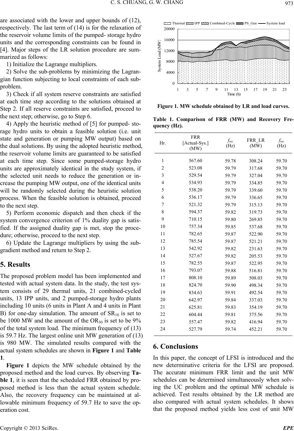 C. S. CHUANG, G. W. CHANG 973 are associated with the lower and upper bounds of (12), respectively. The last term of (14) is for the relaxation of the reservoir volume limits of the pumped- storage hydro units and the corresponding constraints can be found in [4]. Major steps of the LR solution procedure are sum- marized as follows: 1) Initialize the Lagrange multipliers. 2) Solve the sub-problems by minimizing the Lagran- gian function subjecting to local constraints of each sub- problem. 3) Check if all system reserve constraints are satisfied at each time step according to the solutions obtained at Step 2. If all reserve constraints are satisfied, proceed to the next step; otherwise, go to Step 6. 4) Apply the heuristic method of [5] for pumped- sto- rage hydro units to obtain a feasible solution (i.e. unit state and generation or pumping MW output) based on the dual solutions. By using the adopted heuristic method, the reservoir volume limits are guaranteed to be satisfied at each time step. Since some pumped-storage hydro units are approximately identical in the study system, if the selected unit needs to reduce the generation or in- crease the pumping MW output, one of the identical units will be randomly selected during the heuristic solution process. When the feasible solution is obtained, proceed to the next step. 5) Perform economic dispatch and then check if the system convergence criterion of 1% duality gap is satis- fied. If the assigned duality gap is met, stop the proce- dure; otherwise, proceed to the next step. 6) Update the Lagrange multipliers by using the sub- gradient method and return to Step 2. 5. Results The proposed problem model has been implemented and tested with actual system data. In the study, the test sys- tem consists of 29 thermal units, 21 combined-cycled units, 13 IPP units, and 2 pumped-storage hydro plants including 10 units (6 units in Plant A and 4 units in Plant B) for one-day simulation. The amount of SR10 is set to be 1000 MW and the amount of the OR30 is set to be 9% of the total system load. The minimum frequen cy of (13) is 59.7 Hz. The largest online unit MW generation of (13) is 980 MW. The simulated results compared with the actual system schedules are shown in Figure 1 and Table 1. Figure 1 depicts the MW schedule obtained by the proposed method and the load curves. By observing Ta- ble 1, it is seen that the scheduled FRR obtained by pro- posed method is less than the actual system schedule. Also, the recovery frequency can be maintained at al- lowable minimum frequency of 59.7 Hz to save the op- eration cost. 0 4000 8000 12000 16000 20000 1357911131517192123 Time (h) System Load (MW Thermal IPP Combined-Cycle PS_Gen System load Figure 1. MW schedule obtained by LR and load curves. Table 1. Comparison of FRR (MW) and Recovery Fre- quency (Hz). Hr. FRR [Actual-Sys.] (MW) frec (Hz) FRR_LR (MW) frec (Hz) 1 2 3 4 5 6 7 8 9 10 11 12 13 14 15 16 17 18 19 20 21 22 23 24 567.60 523.08 529.54 534.93 538.20 536.17 521.32 594.37 710.15 757.34 782.65 785.54 542.92 527.67 782.55 793.07 808.10 824.70 834.63 642.97 625.81 604.44 557.47 527.79 59.78 59.79 59.79 59.79 59.79 59.79 59.79 59.82 59.80 59.85 59.87 59.87 59.82 59.82 59.87 59.88 59.89 59.90 59.91 59.84 59.83 59.81 59.82 59.74 308.24 317.68 327.04 334.85 339.60 336.65 315.13 319.73 269.85 537.68 522.90 521.21 231.63 205.53 522.95 516.81 508.03 498.34 492.54 337.03 354.19 375.56 416.94 452.21 59.70 59.70 59.70 59.70 59.70 59.70 59.70 59.70 59.70 59.70 59.70 59.70 59.70 59.70 59.70 59.70 59.70 59.70 59.70 59.70 59.70 59.70 59.70 59.70 6. Conclusions In this paper, the concept of LFSI is introduced and the new determinative criteria for the LFSI are proposed. The accurate minimum FRR limit and the unit MW schedules can be determined simultaneously when solv- ing the UC problem and the optimal MW schedule is achieved. Test results obtained by the LR method are also compared with actual system schedules. It shows that the proposed method yields less cost of unit MW Copyright © 2013 SciRes. EPE  C. S. CHUANG, G. W. CHANG Copyright © 2013 SciRes. EPE 974 generation and FFR schedules while the system security is maintained. REFERENCES [1] C. C. Wu and N. Chen, “Online Methodology to Deter- mine Reasonable Spinning Reserve Requirement for Iso- lated Power system,” IEE Proc.-Gene. Transm. and Dis- tri., Vol. 150, No. 4, July 2003, pp. 455-461. [2] C. C. Wu and N. Chen, “Frequency-based Method for Fast-response Reserve Dispatch in Isolated Power Sys- tem,” IEE Proc.-Gene. Transm. and Distri., Vol. 151, No. 1, Jan. 2004, pp. 73-77. [3] G. W. Chang, C. S. Chuang and T. K. Lu, “A Simplified Combined-cycle Unit Model for Mixed Integer Linear Programming-based Unit Commitment,” Proceedings of the 2008 IEEE PES General Meeting, Pittsburgh, PA, USA, July 2008. [4] G. W. Chang, M. Aganagic, J. G. Waight, J. Medina, T. Burton, S. Reeves and M. Christoforidis, “Experiences with Mixed Integer Linear Programming Based Ap- proaches on Short-term Hydro Scheduling,” IEEE Transactions on Power Systems, Vol. 16, No. 4, 2001, pp. 743-749.doi:10.1109/59.962421 [5] X. Guan, P. B. Luh, H. Yan and P. Rogan, “Opti- mization-based Scheduling of Hydrothermal Power Systems with Pumped-storage Units,” IEEE Trans- actions on Power Systems, Vol. 9, No. 2, 1994, pp. 1023-1031.doi:10.1109/59.317641 Nomenclature ,, = Shutdown state of j-th configuration of com- bined-cycle unit i at time step t (binary) t cij z Listed below are notations of variables used in the UC problem formulation throughout the paper. , t ip i u , t ip i p = on/off states of IPP unit i at time step t (binary) = MW purchase of IPP unit i at time step t t i p t = MW output of thermal unit i at time step t , = MW purchase of the segment of the I/O curve of IPP unit i at time step t t ip i p i = Startup state of thermal unit i at time step t (bi- nary) , zi T = Total number of startups/shutdowns of IP P unit i t i z = Shutdown state of thermal unit i at time step t (binary) t = fast-response reserve at time step t (MW) RR t , t ci p t cij y = MW output of combined-cycle unit i at time step t ,, = Startup state of j-th configuration of com- bined-cycle unit i at time step t (binary) ,, pik = on/off pumping state of the pumped-storage unit i within reservoir k at time step t u
|