 Energy and Power Engineering, 2013, 5, 816-823 doi:10.4236/epe.2013.54B157 Published Online July 2013 (http://www.scirp.org/journal/epe) An Interval Probability-based Inexact Two-stage Stochastic Model for Regional Electricity Supply and GHG Mitigation Management under Uncertainty* Yulei Xie, Guohe Huang, Wei Li, Ye Tang North China Electric Power University, Key Laboratory of Regional Energy System Optimization, Ministry of Education, Beijing, China Email: xieyulei850228@yahoo.com, guohe.huang3@gmail.com, weili819@yahoo.com.cn, tye0202@hotmail.com Received October, 2012 ABSTRACT In this study, an interval probability-b ased inexact two -stage stochastic (IP-ITSP) model is develop ed for env ironmental pollutants control and greenhouse gas (GHG) emissions reduction management in regional energy system under uncer- tainties. In the IP-ITSP model, methods of interval probability, interval-parameter programming (IPP) and two-stage stochastic programming (TSP) are introduced into an integer programming framework; the developed model can tackle uncertainties described in terms of interval values an d interval probability d istribution s. The dev eloped mod el is applied to a case of planning GHG -emission mitigation in a regional electricity system, demonstrating that IP-ITSP is applica- ble to reflecting complexities of multi-uncertain ty, and capable of addressing the problem of GHG-emission reduction. 4 scenarios corresponding to different GHG -emission mitigation levels are examined; the results indicates that the model could help decision makers identify desired GHG mitigation policies under various economic costs and envi- ronmental requirements. Keywords: Interval Probability; Inexact Two-stage Stochastic Programming; Electricity Generation; GHG-Mitigation; Energy System 1. Introduction For many decades, the constantly increment of regional electricity demand has forced managers to contemplate and propose ever more comprehensive, complex and ambitious plans for electric power systems. However, most CO2 emissions are emitted mainly from electricity generation processes of burning fossil fuels such as coal, oil and natural gas [1]. A number of impact factors, such as population growth, rapid urbanization and industriali- zation, and global economic development, would inevi- tably result in conflicts among economic objective, elec- tricity demand/supply, and environmental requirement. Moreover, such planning efforts are complicated with a variety of uncertain parameters as well as their interac- tions [2]. It is thus deemed necessary to develop effective optimization methods for supporting regional electric power systems management with GHG-emission mitiga- tion under such complex ities. Previously, a number of mathematical techniques have been introduced to deal with these uncertainties [3-6]. Among these techniques, inexact two stage stochastic programming model (ITSP) integrated with interval pa- rameter programming (IPP) and two stage stochastic programming (TSP) has received extensive attentions to express uncertain parameters with random and dynamic feature as probability distributions and discrete intervals over the past years [7]. Generally, all of the stochastic programming models require probabilistic specifications for uncertain parameters. However, in many practical situations, discrete probability distributions of future events may be predicted using existing statistics and ex- pert judgment. For long run decision making problems, these probabilities are in most cases subjective and diffi- cult to estimate. For example, in electric power manage- ment system, it is often associated with difficulties in acquiring the probability distribution of the random variables/ parameters due to the insufficient available data or the existence of multiple uncertainties. When only limited or imprecise information is available while the stochastic programming method is used, the detailed probabilistic distributions need to be generated based on unrealistic assumptions, resulting in potential errors with the modeling inputs and outputs. Interval probability *Supported by Major Science and Technology Program for Water Pollution Control an d Treatment (NO. 2009Z X 07 631-03). Copyright © 2013 SciRes. EPE 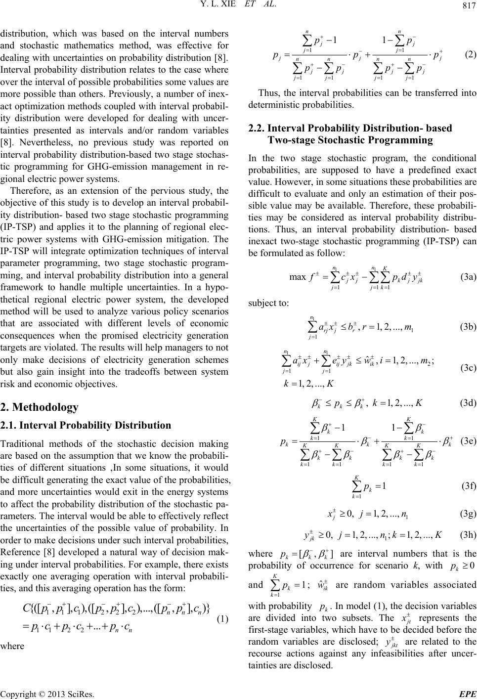 Y. L. XIE ET AL. 817 distribution, which was based on the interval numbers and stochastic mathematics method, was effective for dealing with uncertainties on probability distribution [8]. Interval probability distribution relates to the case where over the interval of possible probab ilities some v alu es are more possible than others. Previously, a number of inex- act optimization methods coupled with interval probabil- ity distribution were developed for dealing with uncer- tainties presented as intervals and/or random variables [8]. Nevertheless, no previous study was reported on interval probability distribution-based two stage stochas- tic programming for GHG-emission management in re- gional electric power systems. Therefore, as an extension of the pervious study, the objective of this study is to develop an interval probabil- ity distribution- based two stage stochastic programming (IP-TSP) and applies it to the planning of regional elec- tric power systems with GHG-emission mitigation. The IP-TSP will integrate optimization techniques of interval parameter programming, two stage stochastic program- ming, and interval probability distribution into a general framework to handle multiple uncertainties. In a hypo- thetical regional electric power system, the developed method will be used to analyze various policy scenarios that are associated with different levels of economic consequences when the promised electricity generation targets are violated. The results will help managers to not only make decisions of electricity generation schemes but also gain insight into the tradeoffs between system risk and economic objectives. 2. Methodology 2.1. Interval Pro ba b il i ty Di s t ri b ut i on Traditional methods of the stochastic decision making are based on the assumption that we know the probabili- ties of different situations ‚In some situations, it would be difficult generating the exact value of the p robabilities, and more uncertainties would exit in the energy systems to affect the probability distribution of the stochastic pa- rameters. The interval would be able to effectively reflect the uncertainties of the possible value of probability. In order to make decisions under such interval probabilities, Reference [8] developed a natural way of decision mak- ing under interval probab ilities. For example, th ere exists exactly one averaging operation with interval probabili- ties, and this averaging operation has the form: 11 122 2 11 22 {([ ,],),([ ,],),...,([ ,],)} ... nn n nn Cppc ppcppc pc pcpc (1) where 11 11 11 11 nn jj jj jj nn nn jj jj jj jj pp pp pp pp p (2) Thus, the interval probabilities can be transferred into deterministic probabilities. 2.2. Interval Prob ab il i ty Di st r ib ut i on - base d Two-stage Stochastic Programming In the two stage stochastic program, the conditional probabilities, are supposed to have a predefined exact value. However, in some situations these probabilities are difficult to evaluate and only an estimation of their pos- sible value may be available. Therefore, these probabili- ties may be considered as interval probability distribu- tions. Thus, an interval probability distribution- based inexact two-stage stochastic programming (IP-TSP) can be formulated as follow: 11 111 max nn K jkj jjk jk cx pdy (3a) subject to: 1 1 1,1, 2,..., n rj jr j axb rm (3b) 11 2 11 ˆ,1, 2,...,; 1, 2,..., nn ij jijjkik jj axeyw im kK (3c) ,1, 2,..., kkk pk K (3d) 11 11 11 11 KK kk kk kk KKKK kk kk kk kk p k (3e) 1 1 K k k p (3f) 1 0,1, 2,..., j j n K ] (3g) 1 0,1, 2,...,;1,2,..., jk yj nk (3h) where , kkk p K are interval numbers that is the probability of occurrence for scenario k, with 0 k p and 11 k k p ; ˆik w are random variables associated with probability k. In model (1), the decision variables are divided into two subsets. The p t represents the first-stage variables, which have to be decided before the random variables are disclosed; kt are related to the recourse actions against any infeasibilities after uncer- tainties are disclosed. y Copyright © 2013 SciRes. EPE  Y. L. XIE ET AL. Copyright © 2013 SciRes. EPE 818 For Model (3), if are considered as uncertain in- puts, the existing methods for solving inexact linear pro- gramming problems cannot be used directly [7]. In this study, an optimized set of targ et values will be identified by having in Model (3) be decision variables. Ac- cordingly, let jjj x x , where jj xx and jt [0,1] ; are decision variables that are used for identifying an optimized set of target values ( ) in order to support the related policy analyses [7]. Accord- ing to Reference [9], the IP-ITSP model can be trans- formed into two deterministic submodels that correspond to the lower and upper bounds of the objective function value, respectively. 3. Application to Ghg-Emission Mitigation in a Regional Electric Power System Consider a typical regional-scale electric power system wherein a manager is responsible for allocating energy resources/services from multiple facilities to multiple end-users through multiple technologies within a plan- ning horizon. The decision maker can formulate the problem as minimizing the expected cost of various en- ergy activities in the region over the planning horizon. Moreover, decision makers always seek to control the emissions of environmental pollutants (e.g., sulfur diox- ide (SO2), nitrogen oxides (NOx), particulate matter (PM)) and greenhouse gas (GHG) in order to meet the regional environmental requirement [10]. In the energy conver- sion sector, every conversion technology has an electric- ity generation target. If the target is not exceeded, a regular cost will be brought to the system; otherwise, the system will be subject to penalties resulted from the extra labor, management, operation and maintenance costs, or capacity expansion and higher costs for imported energy. The future electricity demand during the planning hori- zon is often modeled as an uncertain parameter associ- ated with an interval probability distribution. Most of the other parameters (such as technological efficiency, eco- nomic parameters and utilization factors) are expressed as intervals. Therefore, The FP-ITSP approach is consid- ered appropriate for addressing this planning problem. Table 1 presents the available electricity demands under different interval probability distributions. Electricity generation target, environmental pollutants control and the related economic data are shown in Table 2. Besides, coal-fired power has a residual capacity of 1.0 GW, natural gas-fired power has a residual capacity of 0.28 GW, hydropower has a residual capacity of 0.26 GW. The representative costs and technical data are investi- gated based on governmental reports and other related literature [4-6,10]. Based on a detailed analysis of the study system, four major sets of objectives were considered when modeling this system to achieve the following aims: (a) the lowest cost of purchasing coal, nature gas, crude oil, diesel and gasoline, (b) the lowest operation cost for coal-fired power, gas-fired power, hydropower, wind power, solar power, and nuclear power, (c) the lowest capacity expan- sion cost, and (d) the lowest air pollutant mitigation cost. In detail, the objective functions and constraints were formulated as follows Table 1. The available electricity demands under different interval probability distributions. Demand levels Activity Low Medium High The amount of available electricity [105.00, 125.00][120.00, 145.00] [140.00, 168.00] Probability [0.15, 0.35] [0.45, 0.60] [0.05, 0.15] Table 2. Electricity generation target and the related economic data. Electricity generation target and the related economic data k = 1 k = 2 k = 3 k = 4 k = 5 k = 6 Generation target of each power conversion technology (103GWh) [15, 100] [0, 55] [0, 35] [0, 25] [0, 15] [0, 10] Regular costs for power generation by each power conversion technology ($106/103GWh) [4.00, 6.00] [5.00, 7.00] [5.50, 7.50] [2.50, 3.50] [2.00, 3.00] [10.00, 14.00] Surplus costs for power generation by each power conversion technology ($106/103GWh) [2.00, 3.00] [2.50, 4.50] [3.50, 5.50] [1.50, 2.50] [1.00, 2.00] [6.00, 9.00] Cost of removal SO2 in each power conversion process ($/tonnes) [38.50, 45.50] [32.50, 40.50] 0 0 0 0 Cost of removal NOx in each power conversion process ($/tonnes) [55.50, 75.00] [42.50, 65.50] 0 0 0 0 Cost of removal PM2.5 in each pow er conversion process ($/tonnes) [120.50, 135.50] 0 0 0 0 0  Y. L. XIE ET AL. 819 (1) (2) (3) (4)Minmizef (4a) 1 (1) i I i i PESZ (4b) 111 ()(2) kk KKH kh kkh WPVPPPV p kkh Q k h ,h h )h h h H (4c) 111 (3) km km KMH hkmh kmh YECICp (4d) 11 11 11 (4) () () () KH khkhk k kh KH khkh k kh KH khkh kk kh WpQSOTCTS WpQNOTCTN WpQPMTCTM (4e) subject to: (), ikk kh WZFEQ (4f) [Mass balance for coal] 1 1() K kh kkh WQ ZDTE (4g) max 0, , kkkh WWQ k (4h) 1,,( M kkhk kmhkm m k WQ STRCYECk (4i) [Mass balance for electricity generation] 1 0 integer ,, kmh Ykmh (4j) 1 ,1, v mkmh khY (4k) [Capacity expansion] 1()(1), K kkh kS k WQSOTES h (4l) 1()(1), K kkh kN k WQNOT EN (4m) 1()(1), K kkh k O k WQPMT EPM (4n) 1, kkh K k kWQ COTEMh (4o) [Environmental constraints] ,1,2,..., hhh ph (4p) 11 11 11 11 HH hh hh hh HH HH hh hh hh hh p h (4q) 11 H h h p (4r) where is the expected system cost (million dollar); is the electricity conversion technology, k = 1 for coal-fired power, 2 for natural gas fired power, 3 for hy- dropower, 4 for wind-power, 5 for solar power and 6 for nuclear power; is the capacity expansion option, m =1, 2, 3…, v; is the level of power load, h = 1, 2, 3…, H; i k m h is the energy sources supply (PJ), i = 1 for im- port electricity, i = 2 for coal supply, i = 3 for natural-gas supply, i = 4 hydropower supply, i = 5 for solar power supply, i = 6 for wind power supply, i = 7 for nuclear power supply; i PES is energy sources supply cost ($million/PJ); k PV is the variable cost for converting technologies k; k PP is penalty cost of converting tech- nologies k for excess electricity generation ($million/ GWh); kh Q is the excess power generation by technol- ogy k in scenario h; h is the probability of electricity demand; kmh p Y is the binary variable for technology k with expansion option m; k is the allowable power generation by technology k in load level h; km is the capacity expansion size option m for electricity genera- tion technology k (GW); km is the capital cost for electricity generation technology k expansion size m ($Million/GW); k W IC EC COT is the CO2 emission intensity of power generation technology k (kiloton/GWh); k SOT is the SO2 emission intensity of power generation tech- nology k (kiloton/GWh); k is the NOx emission intensity of power generation technology k (kiloton/ GWh); t NOT PMT is the PM10 emission intensity of power generation technology k (kiloton/GWh); k CTS is the SO2 removal cost of power generation technology k (dol- lar/kiloton); k CTN is the NO2 removal cost of power generation technology k (dollar/kiloton); t CTM is the PM10 removal cost of power generation technology k (dollar/kiloton); k E is the conversion efficiency(TJ/ GWh); h DTE is the electricity demand in load level h (GWh); k is the residual capacity of electricity gen- eration technology k (GW); S RC is the SO2 removal effi- ciency of power generation technology k; is the NOx removal efficiency of power generation technology k; O is the PM10 removal efficiency of power genera- tion technology k; EM is the total allowable CO2 emissions (kiloton); ES is the total allowable SO2 emissions (kiloton); EN is the total allowable NO2 emissions (kiloton); EPM is the total allowable PM10 emissions in period t (kiloton). Copyright © 2013 SciRes. EPE 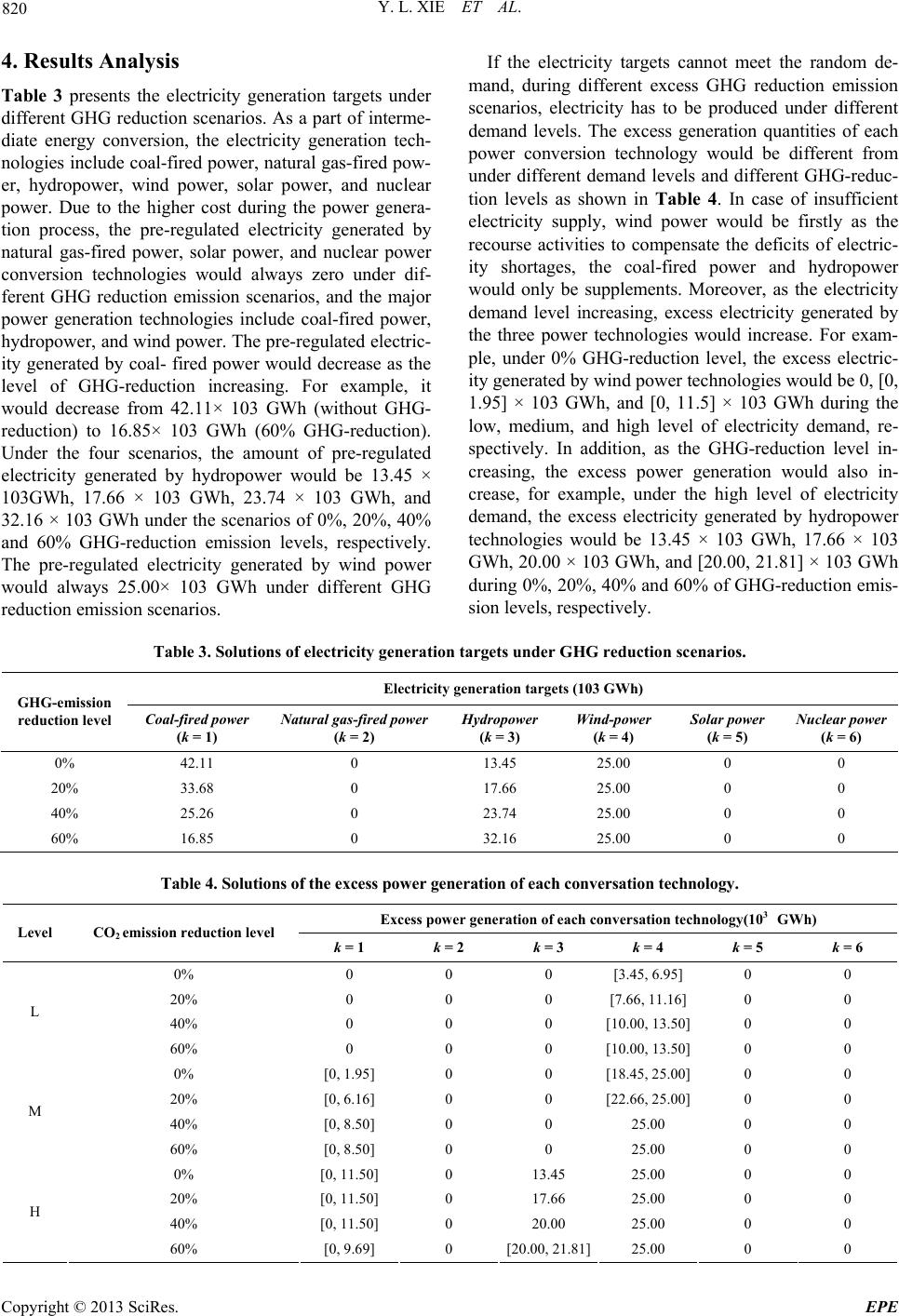 Y. L. XIE ET AL. 820 4. Results Analysis Table 3 presents the electricity generation targets under different GHG reduction scenarios. As a part of interme- diate energy conversion, the electricity generation tech- nologies in clude coal-fired power, n atural gas-fired pow- er, hydropower, wind power, solar power, and nuclear power. Due to the higher cost during the power genera- tion process, the pre-regulated electricity generated by natural gas-fired power, solar power, and nuclear power conversion technologies would always zero under dif- ferent GHG reduction emission scenarios, and the major power generation technologies include coal-fired power, hydropower, an d wind power. The pre- regulated electric- ity generated by coal- fired power would decrease as the level of GHG-reduction increasing. For example, it would decrease from 42.11× 10³ GWh (without GHG- reduction) to 16.85× 10³ GWh (60% GHG-reduction). Under the four scenarios, the amount of pre-regulated electricity generated by hydropower would be 13.45 × 10³GWh, 17.66 × 10³ GWh, 23.74 × 10³ GWh, and 32.16 × 10³ GWh under the scenarios of 0%, 20%, 40% and 60% GHG-reduction emission levels, respectively. The pre-regulated electricity generated by wind power would always 25.00× 10³ GWh under different GHG reduction emission scenarios. If the electricity targets cannot meet the random de- mand, during different excess GHG reduction emission scenarios, electricity has to be produced under different demand levels. The excess generation quantities of each power conversion technology would be different from under different demand levels and different GHG-reduc- tion levels as shown in Table 4. In case of insufficient electricity supply, wind power would be firstly as the recourse activities to compensate the deficits of electric- ity shortages, the coal-fired power and hydropower would only be supplements. Moreover, as the electricity demand level increasing, excess electricity generated by the three power technologies would increase. For exam- ple, under 0% GHG-reduction level, the excess electric- ity generated by wind power technologies would be 0, [0, 1.95] × 103 GWh, and [0, 11.5] × 103 GWh during the low, medium, and high level of electricity demand, re- spectively. In addition, as the GHG-reduction level in- creasing, the excess power generation would also in- crease, for example, under the high level of electricity demand, the excess electricity generated by hydropower technologies would be 13.45 × 10³ GWh, 17.66 × 10³ GWh, 20.00 × 10³ GWh, an d [20.00, 21.81] × 103 GWh during 0%, 20%, 40% and 60% of GHG-reduction emis- sion levels, respectively. Table 3. Solutions of electricity generation targets under GHG reduction scenarios. Electricity generation targets (103 GWh) GHG-emission reduction level Coal-fired power (k = 1) Natural gas-fired power (k = 2) Hydropower (k = 3) Wind-power (k = 4) Solar power (k = 5) Nuclear power (k = 6) 0% 42.11 0 13.45 25.00 0 0 20% 33.68 0 17.66 25.00 0 0 40% 25.26 0 23.74 25.00 0 0 60% 16.85 0 32.16 25.00 0 0 Table 4. Solutions of th e excess power generation of each con versation technology. Excess power generation of each conversation technology(103 GWh) Level CO2 emission reduction level k = 1 k = 2 k = 3 k = 4 k = 5 k = 6 0% 0 0 0 [3.45, 6.95] 0 0 20% 0 0 0 [7.66, 11.16] 0 0 40% 0 0 0 [10.00, 13.50] 0 0 L 60% 0 0 0 [10.00, 13.50] 0 0 0% [0, 1.95] 0 0 [18.45, 25.00] 0 0 20% [0, 6.16] 0 0 [22.66, 25.00] 0 0 40% [0, 8.50] 0 0 25.00 0 0 M 60% [0, 8.50] 0 0 25.00 0 0 0% [0, 11.50] 0 13.45 25.00 0 0 20% [0, 11.50] 0 17.66 25.00 0 0 40% [0, 11.50] 0 20.00 25.00 0 0 H 60% [0, 9.69] 0 [20.00, 21.81]25.00 0 0 C opyright © 2013 SciRes. EPE 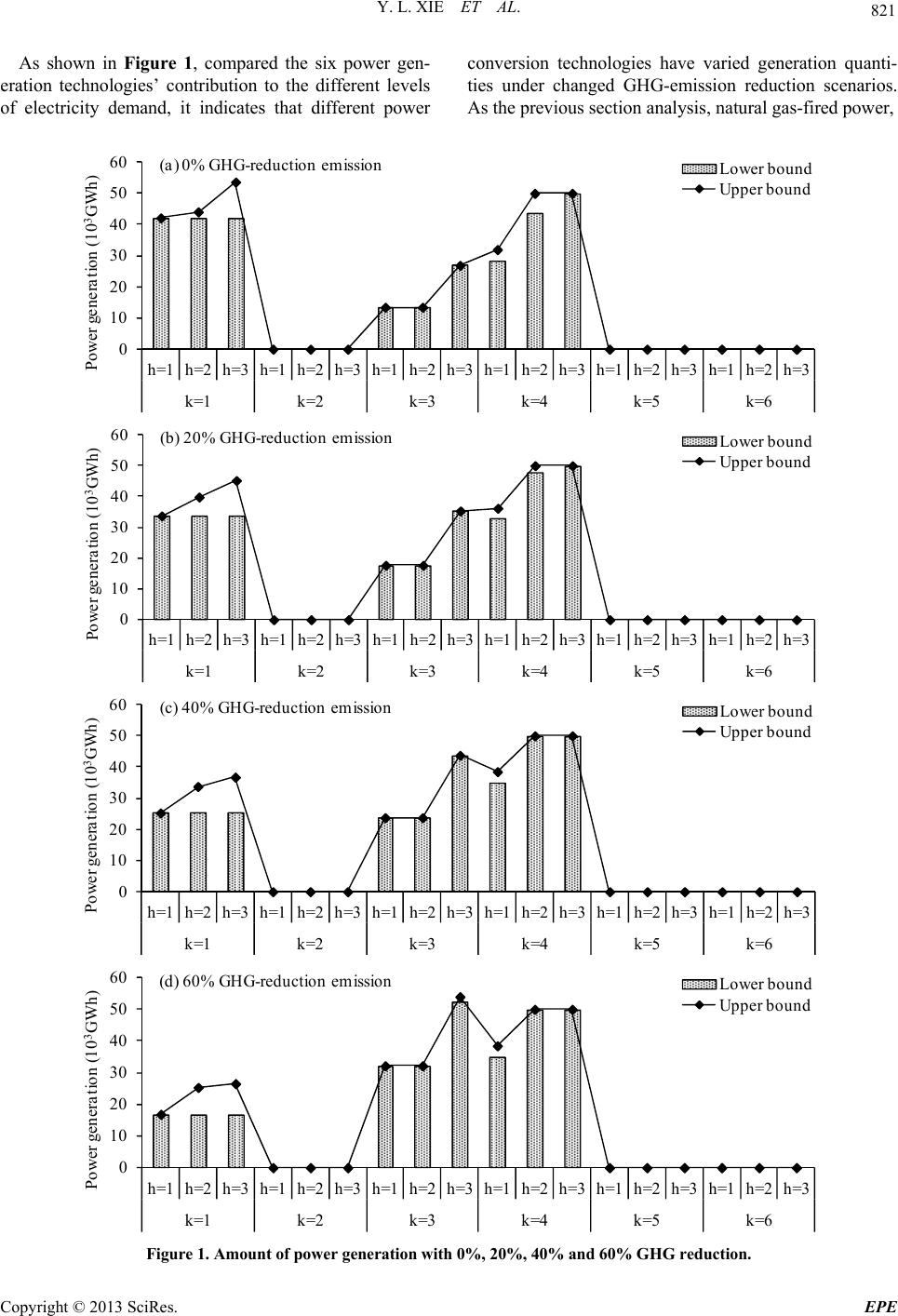 Y. L. XIE ET AL. 821 As shown in Figure 1, compared the six power gen- eration technologies’ contribution to the different levels of electricity demand, it indicates that different power conversion technologies have varied generation quanti- ties under changed GHG-emission reduction scenarios. As the previous section analysis, natural gas -fire d p owe r, 0 10 20 30 40 50 60 h=1h=2h=3h=1h=2h=3h=1h=2h=3h=1h=2h=3h=1 h=2 h=3 h=1 h=2 h=3 k=1k=2k=3k=4k=5 k=6 Power ge neration (10 3 GWh) (a) 0% GHG -r educti on emis si onL ower bound Upper bound 0 10 20 30 40 50 60 h=1h=2h=3 h=1h=2h=3 h=1h=2h=3h=1 h=2 h=3 h=1h=2 h=3h=1h=2h=3 k=1k=2k=3k=4 k=5 k=6 Power generation (10 3 GWh) (b ) 20% GHG-re duction emissionL ower bound Upper bound 0 10 20 30 40 50 60 h=1h=2h=3h=1h=2h=3h=1h=2h=3 h=1 h=2 h=3 h=1 h=2 h=3 h=1h=2h=3 k=1k=2 k=3 k=4 k=5k=6 Power generation (103GWh) (c) 40% GHG-reduc tion emissionL ower bou nd Up pe r bound 0 10 20 30 40 50 60 h=1h=2h=3 h=1 h=2 h=3 h=1 h=2 h=3 h=1 h=2h=3 h=1 h=2 h=3 h=1 h=2 h=3 k=1k=2k=3k=4k=5 k=6 Power generation (10 3 GWh) (d) 60% GHG-re duc t ion emis sionL ower bound Up pe r bound Figure 1. Amount of power generation with 0%, 20%, 40% and 60% GHG reduction. C opyright © 2013 SciRes. EPE 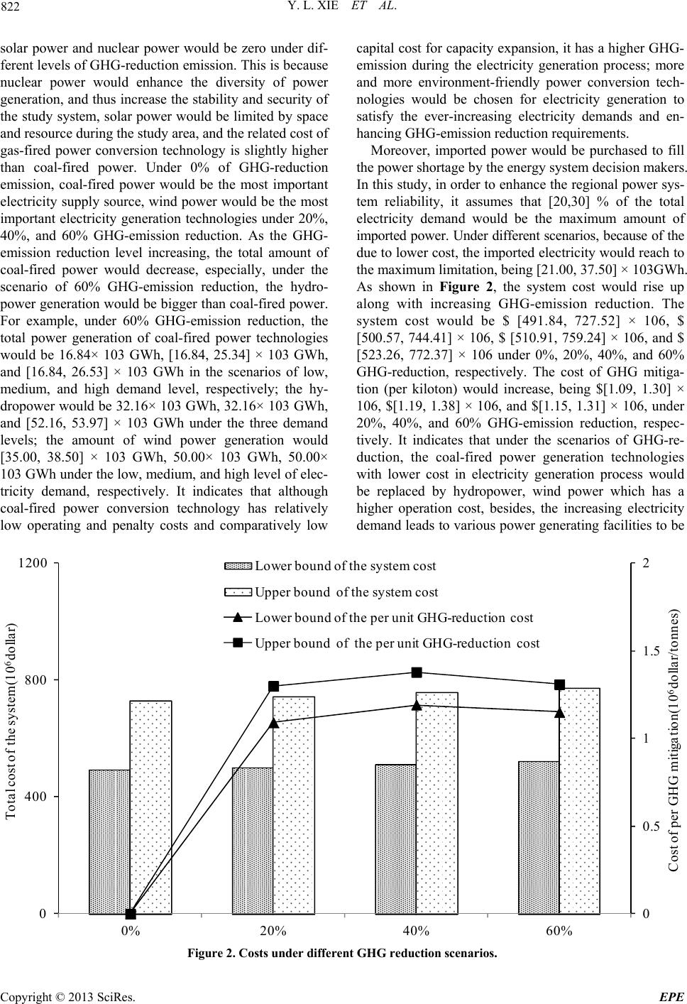 Y. L. XIE ET AL. 822 solar power and nuclear power would be zero under dif- ferent levels of GHG-reduction emission. This is because nuclear power would enhance the diversity of power generation, and thus increase the stability and security of the study system, solar power would be limited by space and resource during the study area, and the related cost of gas-fired power conversion technology is slightly higher than coal-fired power. Under 0% of GHG-reduction emission, coal-fired power would be the most important electricity supply source, wind power would be the most important electricity generation technologies under 20%, 40%, and 60% GHG-emission reduction. As the GHG- emission reduction level increasing, the total amount of coal-fired power would decrease, especially, under the scenario of 60% GHG-emission reduction, the hydro- power generation would be bigger than coal-fired power. For example, under 60% GHG-emission reduction, the total power generation of coal-fired power technologies would be 16.84× 10³ GWh, [16.84, 25.34] × 103 GWh, and [16.84, 26.53] × 103 GWh in the scenarios of low, medium, and high demand level, respectively; the hy- dropower would be 32.16× 10³ GWh, 32.16× 10³ GWh, and [52.16, 53.97] × 103 GWh under the three demand levels; the amount of wind power generation would [35.00, 38.50] × 103 GWh, 50.00× 10³ GWh, 50.00× 10³ GWh under the low, medium, and h igh level of elec- tricity demand, respectively. It indicates that although coal-fired power conversion technology has relatively low operating and penalty costs and comparatively low capital cost for capacity expansion, it has a higher GHG- emission during the electricity generation process; more and more environment-friendly power conversion tech- nologies would be chosen for electricity generation to satisfy the ever-increasing electricity demands and en- hancing GHG-emission reduction requirements. Moreover, imported power would be purchased to fill the power shortage by the energy system decision makers. In this study, in order to enhance the regional power sys- tem reliability, it assumes that [20,30] % of the total electricity demand would be the maximum amount of imported power. Under different scenarios, because of the due to lower cost, the imported electricity would reach to the maximum limitation, being [21.00, 37.50] × 103GWh. As shown in Figure 2, the system cost would rise up along with increasing GHG-emission reduction. The system cost would be $ [491.84, 727.52] × 106, $ [500.57, 744.41] × 106, $ [510.91, 759.24] × 106, and $ [523.26, 772.37] × 106 under 0%, 20%, 40%, and 60% GHG-reduction, respectively. The cost of GHG mitiga- tion (per kiloton) would increase, being $[1.09, 1.30] × 106, $[1.19, 1.38] × 106, and $[1.15, 1.31] × 106, under 20%, 40%, and 60% GHG-emission reduction, respec- tively. It indicates that under the scenarios of GHG-re- duction, the coal-fired power generation technologies with lower cost in electricity generation process would be replaced by hydropower, wind power which has a higher operation cost, besides, the increasing electricity demand leads to various power generating facilities to be 0 0.5 1 1.5 2 0 400 800 1200 0%20% 40% 60% C o s t o f p e r GHG m it igat io n (10 6 dollar/tonnes) Total cost of the system(10 6 doll ar) Low er bound of the system cost Upper bound of the system cost L ower bound of t he per unit GH G-re duc t ion cost Upper bound of the pe r unit GHG-reduct ion cost Figure 2. Costs under different GHG red uction scenarios. C opyright © 2013 SciRes. EPE  Y. L. XIE ET AL. 823 expanded, bringing about a high capital cost. 5. Conclusion An interval probability-based inexact two-stage stochas- tic (IP-ITSP) model is developed for regional electricity system and greenhouse gas (GHG) emissions reduction management under uncertainties. The method is based on interval probability, interval-parameter programming (IPP) and two-stage stochastic programming (TSP). Un- certainties in the energy system could present as both interval probability distributions and interval values to be incorporated within a general optimization framework. The developed model is applied to a case of planning GHG-emission mitigation in a regional electricity system, demonstrating that IP-ITSP is applicable to reflecting complexities of multi-uncertainty, and capable of ad- dressing the problem of GHG-emission reduction. 4 sce- narios corresponding to different GHG -emission mitiga- tion levels are examined; Solutions provide an effective linkage between the predefined environmental policies and the associated economic implications (e.g., losses and penalties caused by improper policies). The solutions contain a combination of deterministic, interval and dis- tributional information, and can thus facilitate the reflec- tion for different forms of uncertainties. The results indi- cate that the model can help managers obtain multiple decision alternatives, as well as provide bases for further analyses of tradeoffs between energy management cost and GHG-emission reduction. REFERENCES [1] C. B. Field and M. R. Raupach, “The Global Carbon Cy- cle: Integrating Humans, Climate, and the Natural World,” Island Press, 2004. [2] IPCC, “Climate Change Contribution of Working Group I to the Fourth Assessment Report of the IntergovernMen- tal Panel on Climate Change,” Cambridge, United King- dom/New York, NY, USA: Cambridge University Press, 2007. [3] S. E. Fleten and T. K. Kristoffersen, “Short-term Hydro- Power Production Planning by Stochastic Programming,” Computers and Operations Research, Vol. 35, No. 8, 2008, pp. 2656-2671. doi:10.1016/j.cor.2006.12.022 [4] Q. G. Lin and G. H. Huang, “IPEM: An inter- val-parameter energy systems planning model,” Energy Sources A: Recovery, Utilization, and Environmental Ef- fects, Vol.30, No.14, 2008, pp.1382-1399. doi:10.1080/15567030801929043 [5] Y.Y. Liu, “A dynamic two-stage energy systems planning model for Saskatchewan, Canada,” M. S. Dissertation, Faculty of Graduate Studies and Research, Regina, Sas- katchewan, Canada. 2007. [6] L. Liu, G. H. Huang, G. A. Fuller, A. Chakma and H. C. Guo, “A Dynamic Optimization Approach for Nonre- newable Energy Resources Management Under Uncer- tainty,” Journal of Petroleum Science and Engineering, Vol. 26, 2000, pp. 301-309. doi:10.1016/S0920-4105(00)00044-9 [7] Y. P. Li, G. H. Huang, S. L. Nie, X. H. Nie and I. Maqsood, “An Interval-parameter Two-stage Stochastic Integer Programming Model for Environmental Systems Planning under Uncertainty,” Engineering Optimization, Vol. 38, No. 4, 2006, pp. 461-483. doi:10.1080/03052150600557742 [8] R. R. Yager, “Decision Making under Interval Probabili- ties,” International Journal of Appeoximate Reasoning, Vol. 22, No. 3, 1999, pp. 195-215. doi:10.1016/S0888-613X(99)00028-6 [9] G. H. Huang and D. P. Loucks, “An Inexact Two-stage Stochastic Programming Model for Water Resources Management under Uncertainty,” Civil Engineering and Environmental Systems, Vol. 17, 2000, pp. 95-118. doi:10.1080/02630250008970277 [10] Y. L. Xie, Y. P. Li, G. H. Huang and Y. F. Li, “An Inter- val Fixed-mix Stochastic Programming Method for Greenhouse Gas Mitigation in Energy Systems under Uncertainty,” Energy, Vol. 35, 2010, pp. 4627-4644. doi:10.1016/j.energy.2010.09.045 C opyright © 2013 SciRes. EPE
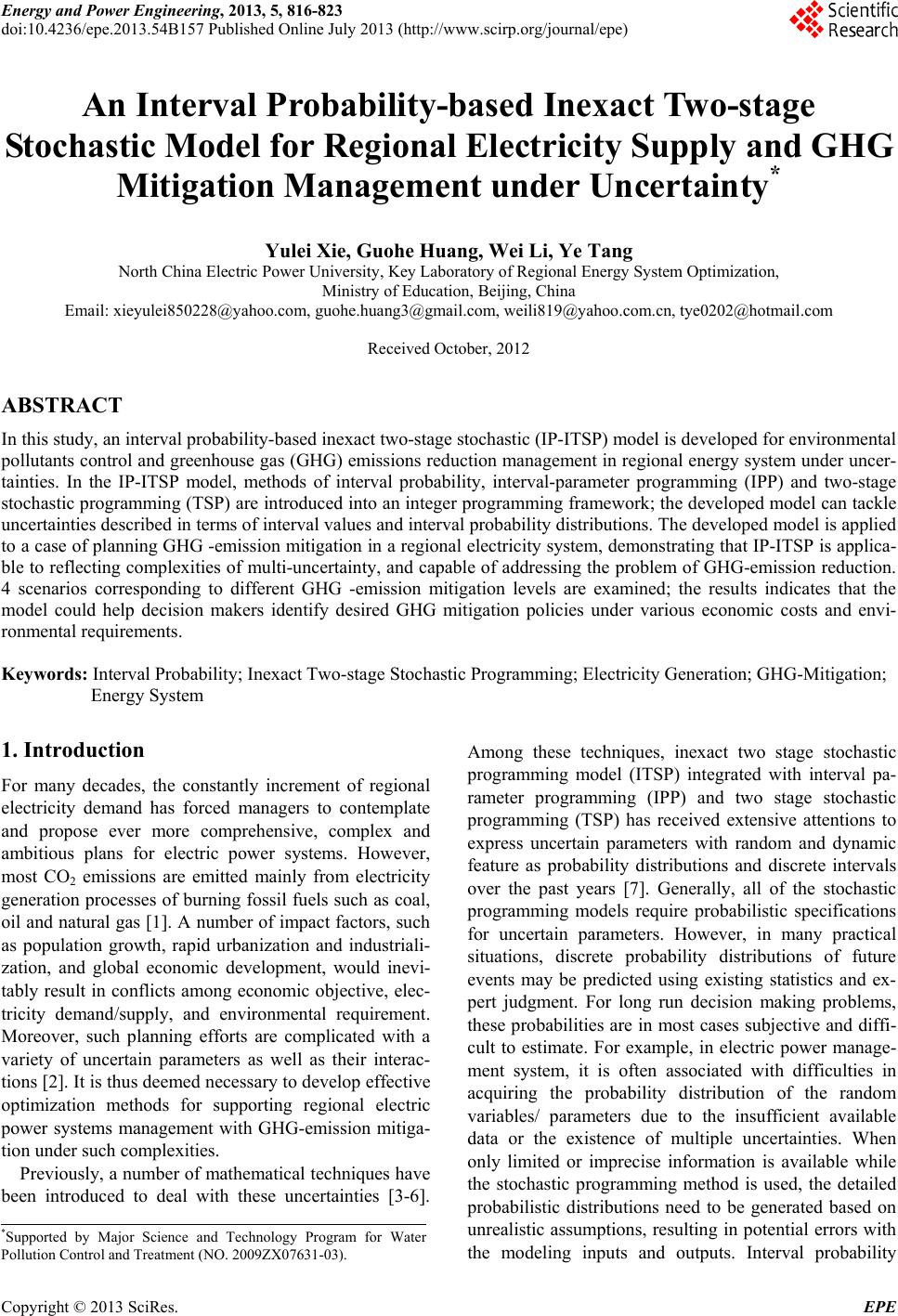
|