International Journal of Geosciences, 2011, 2, 13-28
doi:10.4236/ijg.2011.21002 Published Online February 2011 (http://www.SciRP.org/journal/ijg)
On the Wind and Turbulence in the Lower Atmosphere
above Complex Terrain
George Jandieri1, Alexander Surmava2, Anzor Gvelesiani2
1Georgian Techni cal Universit y , Institute of Cybernetics, Tbilisi, Georgia
2M. Nodia Institute of Geophysics, Tbilisi, Georgia
Received November 18, 2010; revised December 20, 2010; accepted De c ember 23, 2010
Abstract
Numerical modeling and studies of the wind fields at the junction of three continents: over the complex ter-
rains of the South-east Europe, Asia Minor, Middle East, Caucasus and over the Black, Caspian and Medi-
terranean seas have been carried out for the first time. Traveling synoptic scale vortex wave generation and
subsequent evolution of orographic vortices are discovered. Wind fields, spatial distribution of the coeffi-
cients of subgrid scale horizontal and vertical turbulence and the Richardson number are calculated. It is
shown that the local relief, atmospheric hydrothermodynamics and air-proof tropopause facilitate the genera-
tion of

-mesoscale vortex and turbulence amplification in the vicinity of the atmospheric boundary layer
and tropopause. Also turbulence parameters distribution in the troposphere has the same nature as in the
stratosphere and mesosphere: turbulence coefficients, stratification of the vertical profiles of the Richardson
number, thickness of the turbulent and laminar layers.
Keywords: Numerical Modeling, Complex Terrain, Characteristics of Atmospheric Turbulence, Wind Field,
Mesoscale Vortex, Bulk Richardson Number
1. Introduction
At present many hydrometeorologists are actively study-
ing mesoscale atmospheric processes above the complex
terrains. The problem is complex and its solution is
closely related to other important problems of dynamical
meteorology, including a problem of atmospheric turbu-
lence of different scales in the mountainous regions.
Boundary-layer studies of mountainous terrain have
mainly focused on global characteristics, such as thermal
stratification, boundary-layer growth rates, circulation
patterns and valley winds. The relatively few studies
devoted to the turbulence structure over non-flat terrain
have mainly been restricted to comparatively gentle h ills.
In [1], the nature of turbulent kinetic energy in a steep
and narrow Alpine valley in Switzerland under fair-
weather summertime conditions was investigated for a
detailed case study, in which the evaluation of aircraft
data was combin ed with the ap plication of h igh-resolution
large-eddy simulations using the numerical model ARPS.
Excellent correlation was established between surface
heat flux and the up-valley wind speed. The measure-
ments and simulations show that despite the complexity
of the terrain and the apparent differences from a classi-
cal convective boundary layer, the turbulence structure
reveals reproducible patterns and scaling characteristics.
Generalization of obtained results by [1] requires an in-
vestigation of other valley geometries and different to-
pographic orientations. In particular, further investigation
of the functional dependence between up-valley wind
speed and local surface fluxes. The authors of paper [2]
studied vertical winds and turbulence in the troposphere
in mountain-wave conditions near Kiruna in Arctic Swe-
den. They show that the horizontal and vertical wave-
lengths of the dominating mountain-waves were ~10 - 20
km, the amplitudes in vertical wind 1-2 1
ms


, and
turbulence velocities below 5500 m height were about
40% of the time during winter months. This is a much
higher rate than the Advanced Research and Weather
Forecasting model (WRF) predictions for conditions of
Richardson number 1Ri

but similar to WRF predic-
tions of 2Ri

. The cause of low Ri is a combination
of wind-shear at synoptic upper-level fronts and pertur-
bations in static stability due to the mountain-waves.

G. JANDIERI ET AL.
14
Comparison with radiosondes suggests that WRF under-
estimates wind-shear and the occurrence of thin layers
with very low static stability, so that vertical mixing by
turbulence associated with mountain waves may be sig-
nificantly more than suggested by the model. A statistical
correlation between enhanced turbulence and gravity
waves was noted in [3].
The authors [4] investigating turbulence of a neutral
atmosphere at different heights obtained the following
results: 1) Radar observations of the mesosphere, air-
crafts smoke trails into the stratosphere, radar observa-
tions of thin layers in the troposphere and lower strato-
sphere show that layered and stratified phenomena are
common in the atmosphere. It was shown that “cat’s-eye”
structures are not uncommon in the atmosphere as a pre-
cursor to turbulence breakdown and such structures are
often associated with Kelvin-Helmholtz (K-H) billows.
Authors of [5] have indicated that other mechanism, such
as the Holmboe instability, can also generate such struc-
tures. K-H instabilities are only dominant in weak ly stra-
tified flows, whereas the Holmboe instability is more
likely in strongly stratified flows. There can be occasions
when other mechanisms of breakdown can be responsi-
ble for the turbulence. The formation of cat’s-eye struc-
tures is only one possible mechanism. Cat’s-eye struc-
tures are visually impressive, so they tend to dominate
the literature, but it is not clear whether they are in fact
the main mode of turbulence breakdown at all. 2) By
using radars and various specialized techniques they
have also obtained information at smaller scales (~1 m -
100 m).Turbulence is considered here to be generally the
result of a non-linear breakdown of larger, more organ-
ized structures which have become unstable, with scales
comparable to or larger than the buoyancy scale.
A number of remote-sensing wind-measuring instru-
ments such as LIDAR and radar wind profilers [6] have
been used for monitoring of low-level wind shear and
turbulence. Data collected in a field experiment of the
radio metering conducted in Hong Kong in February
2006 were used to obtain the Richardson number profile
up to 1.5 km above ground. The Richar dson number pro-
files are found to capture the turbulence events reasona-
bly well. The atmospheric condition was favorable for
the generation of turbulence when 0.25
c
Ri Ri . It
was also noted that, at the above four times, the Ri
number could be less than 0.25 below 400 m or so, espe-
cially the occurrence of negative Ri value. This feature
is mainly related to turbulent airflow associated with
thermodynamic instability near the ground. Downstream
of the airflow, there are a number of waves/vortices be-
tween 700 and 1600 m high with the dimensions of sev-
eral hundred meters in height and a couple of kilometers
horizontally. A possible reason of turbulence is the shear
instability associated with quick veering of the wind with
height.
Meteorological researchers have made efforts to im-
prove the stability description of a moist atmosphere by
using variations of the Richardson number [7]. The
Richardson number is often used as an important index
for judging shearing instability and symmetry in stability:
the conventional baroclinic instabilities dominate if
0.95Ri , symmetry instabilities dominate if 0.25

0.95Ri

, and Kelvin-Helmholtz instabilities dominate
if 0.5Ri

. A new Richardson number is defined for
describing the stability of a mo ist atmosphere (*
Ri ). The
results show that convective instability is co ncentrated in
the lower troposphere while instability determined by
*1Ri

is mainly located in the middle and upper tro-
posphere above the rainfall areas, may be used to indi-
cate and estimate the rainfall occurrence and develop-
ment. Richardson numbers in the three thermodynamic
states of the atmosphere can be obtained when potential
temperature,

(of dry atmosphere), equivalent poten-
tial temperature, e

(saturated moist region), and gen-
eralized potential temperature, *

, are applied to calcu-
late Brunt-Väisälä frequency, respectively.
In [8] spectral and structure function analyses of hori-
zontal velocity fields observed in the upper troposphere
and lower stratosphere during the Severe Clear Air Tur-
bulence Collides with Air Traffic (SCATCAT) field
program, conducted over the Pacific, were carried out to
identify the scale interactions of turbulence and small
scale gravity waves. In the presence of turbulence, tran-
sitional power spectra from 2
k to 5/3 k were found to
be associated with the gravity waves and turbulence,
respectively. The second-order structure function analy-
sis was able to translate these spectral slopes into r and
2/3
r, consistent with Monin-Yaglom conversion law, in
physical space, which presented clearer pictures of scale
interactions between turbulence and gravity waves. The
third-order structure function analysis indicated the exis-
tence of a narrow region of inverse energy cascade from
the scales of turbulence up to the gravity waves scales.
This inverse energy cascade region was linked to the
occurrence of Kelvin-Helmholtz instability and other
wave-amplifying mechanisms, which were conjectured
to lead to the breaking of small-scale gravity waves and
the ensuing generation of turbulence. The multifractal
analyses revealed further scale breaks between gravity
waves and turbu len ce. In [9 ] it is shown with a numerical
simulation that a sharp increase in the vertical tempera-
ture gradient and Brunt-Väisälä frequency near the tro-
popause may produce an increase in the amplitudes of
internal gravity waves propagating upward from the tro-
posphere, wave breaking and generation of stronger tur-
bulence. Turbulent diffusion coefficient calculated nu-

G. JANDIERI ET AL.
15
merically and measured with MU radar are of 1 - 10
21
ms

in different seasons in Shigaraki, Japan (35˚N,
136˚E). These values lead to the estimation of vertical
ozone flux from the stratosphere to the troposphere of
14
(110) 10 21 ms

 which may substantially add to th e
usually supposed ozone downward transport with the
general atmospheric circulation. Therefore, local en-
hancements of IGW intensity and turbulence at tropo-
spheric heights over the mountains due to their oro-
graphic excitation may lead to the changes in tropo-
spheric and total ozone over different regions. In [10]
high resolution (150 m) wind measurements by Meso-
sphere-Stratosphere-Troposphere (MST) radar and by
Lower Atmospheric Wind Profiler (LAWP) have been
used to study variation of turbulence intensity. Layers of
higher turbulence are observed in the lowe r stratosph ere.
The heights of the turbulent layers in the lower strato-
sphere do not correlate with the levels of minimum
Richardson number. During the short-period gravity
wave activity (~7 h) the high frequency convectively
generated gravity waves breakdown generates the ob-
served turbulence layers. A non-linear interaction be-
tween the waves of different scales might be responsible
for the breakdown and generation of turbulence layers. It
should be noted that different mechanisms of wave
breaking can coexist and complement each other. From
the above it follows that there are many unresolved
problems related to the hydrodynamic interaction of air
with a complex terrain.
The objective of this paper is theoretical investigation
of the features of hydrodynamic interaction of the at-
mosphere with complex terrain at the junction of three
continents: Sou th-eastern Europe, Asia Minor and Africa,
where there are located several large seas-the eastern part
of the Mediterranean sea, the Black, Azov and Caspian
seas, etc, many high mountain ranges, forests, steppes
and deserts stretched a hundred kilometers. The evolu-
tion of the wave of cyclonic and anticyclonic vortices
and the obtained mesoscale air flow for the considered
complex terrain is modeled for the first time. We use a
regional model of the atmospheric processes elaborated
at the M. Nodia Institute of Geophysics [11].
2. Formulation of the Problem
2.1. Basic Equations
Basic equations of the model describing variations of the
meteorological fields are:
1) for the tropospher e [12,13]:

2
d1
10.61
d
uPz u
lv gqu
txx h
 



 

,

2
d1
10.61
d
vPz v
lu gqv
tyy h
 



 

,

10.61
gqh
RT




, 1d 0
huhvhwh wh
txy dz


 

 
 
,
2
1con
p
L
uvwSw
txyC t h

 
 



 

 
,
1con qqqqq Q
uvw q
txy t




 
 
, 22
x
y


 

,
con
mmmmm N
uvw m
txy t




 
 

 
, (1)
zzz
wuvwh
txy

 

, zh



, duvw
dt txy


 
 


,
2) for the active layer of soil [14,15]:



EC
CC
DC
tzz z

 

, 2
2
s
oil soil
soil
TT
K
tz


 at 0
s
oil
zZ

 , (2)
3) for the layer of sea water [14]:
2
2
1
sea sea
sea sea sea
TT
I
K
tCz z 



 , at 0
s
ea
zZ

 , (3)

G. JANDIERI ET AL.
16
where t is time; x, y, and z are the axes of the Cartesian
coordinate directed to the east, north and vertically up-
wards, respectively;

zh   is the dimensionless
vertical coordinate;

0,50xy
 
m is the surface
layer height; 0

is the height of the relief;


,,
H
txy
is the height of the tropopause; hH

; u, v, w, and
w are the wind velocity components along the axes x, y, z,
and

, respectively; TT 

, and


PPz 

 are
the analogues of temperature and pressure, respectively;
300TK; T and P are the devotions of tempera-
ture and pressure from the standard vertical distributions
 
,,, ,,,,,,TtxyzTtxyz TzTtxyz 
,
 
,,, ,,,,,,PtxyzPtxyzPzPtxyz
; T and P
are the temperature and pressure of the atmosphere, re-
spectively: Tz

 and

Pz are the standard verti-
cal distributions of the temperature and pressure, respec-
tively;

is the standard vertical temperature gradient;
T and P are the background deviations of the tem-
perature and pressure from standard vertical distributions;

and

are the mesoscale and background compo-
nents of the analogue of temperature, respectively;


; q and Q are the mass fraction of water va-
pour and the background mass fraction of water vapour,
respectively; qqQ
; m and M are the mass fraction
of cloud water and the background mass of cloud water,
respectively; mmM
 ;
s
oil
T and
s
ea
T are the tem-
peratures of soil and seawater, respectively; C is the vo-
lume content of soil water;

z  and
s
ea

are the
standard vertical distributions of the densities of dry air
and seawater, respectively; 1;dp dz 

 g is the
gravitational acceleration; R is the universal gas constant
for dry air;
p
C and
s
ea
C are the specific heat capacities
of dry air at constant pressure and seawater, respectively;
S is the thermal stability parameter; L is the latent heat of
condensation; con

is the condensation rate; Nt

 is
the intensity of prescription;

cr
Nt mmt

 
when cr mm, and 0 when cr mm [14]; cr m is the
critical magnitude of the mass fraction of a cloud water;
t

is the time of setting out of a surplus cloud water; D
is the diffusion coefficient of water in soil; E is the filtra-
tion coefficient of water in soil;
s
ea
I
is the total solar
radiation flux in sea water;
s
oil
K
and
s
ea
K
are the
thermal diffusivity coefficients of soil and sea water,
respectively;

and

are the horizontal and vertical
turbulent diffusion coefficients.
The set of Equations (1) and (2), (3) are solved in the
coordinate systems


,,,txy

and

,,,txyz , respec-
tively.The initial and boundary conditions, the values of
background fields and methods of parameterization of
the separate meteorological processes are selected in
accordance with specific objectives of modeling.
2.2. Boundary and Initial Conditions, the Main
Parameters of the Regional Problem
The boundary and initial conditions for the set of Equa-
tions (1-3) according to [13,16,17] are:
2.2.1. Verti c al Boundary C o ndi ti ons
1) for the system (1):
    
1
0, 0,,,,,0,,wtxygRThtxy hxy
 

 
, at 1

,


00
00 0
00
,,
,,
,0,
uv
AV uhAV vh
m
AVhAV mh
qAV qqhw













 






   




 
 



at 0

, (4)
2) for systems (2) and (3):
 
00
e
ee epeqee
T
CKC AVTTLAVqqI
z
 



1
0
1
0
,atd0
,atd 0
por
we
CC Nt
C
DAVqq Nt
z












, at 0 z


, (5)
0
e
TC
zz



 at 02zm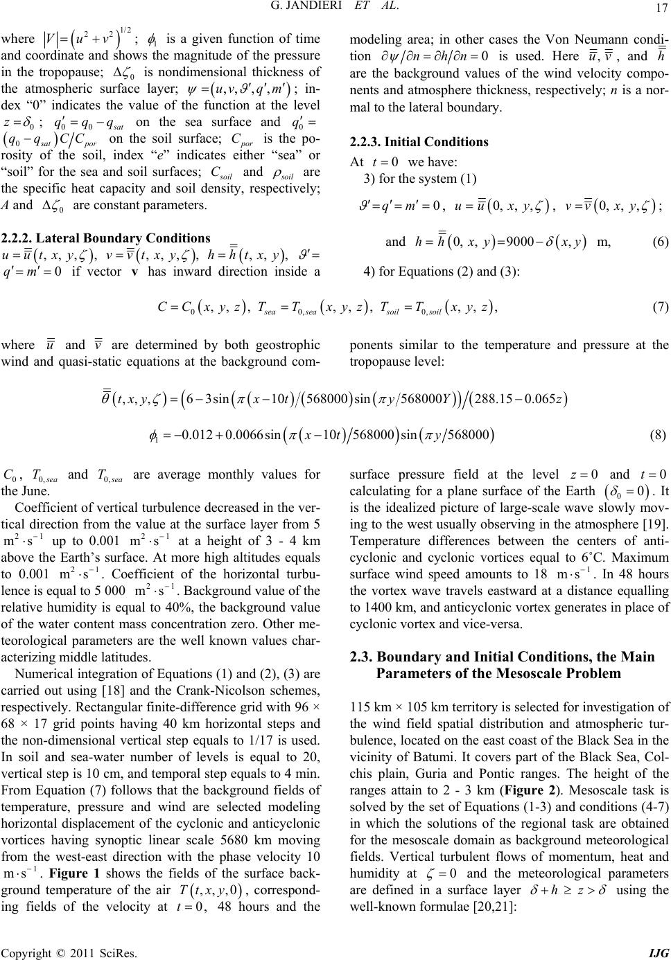


,

G. JANDIERI ET AL.
17
where

1/2
22
Vuv ; 1

is a given function of time
and coordinate and shows the magnitude of the pressure
in the tropopause; 0

 is nondimensional thickness of
the atmospheric surface layer;

,,, ,uvq m 
 
; in-
dex “0” indicates the value of the function at the level
0
z

; 00
s
at
qqq
 on the sea surface and 0
q



0
s
at por
qqCC on the soil surface;
p
or
C is the po-
rosity of the soil, index “e” indicates either “sea” or
“soil” for the sea and soil surfaces;
s
oil
C and
s
oil

are
the specific heat capacity and soil density, respectively;
A and 0

 are constant parameters.
2.2.2. Later al B oundary Conditi on s

,,,uutxy

,

,,,vvtxy

,

,,hhtxy,



0qm

 if vector v has inward direction inside a
modeling area; in other cases the Von Neumann condi-
tion 0nhn


  is used. Here ,uv, and h
are the background values of the wind velocity compo-
nents and atmosphere thickness, respectively; n is a nor-
mal to the lateral boundary.
2.2.3. Initial Conditions
At 0t

we have:
3) for the system (1)
0qm




,


0, ,,uuxy

,

0, ,,vv xy

;
and
 
0, ,9000,hh xyxy   m, (6)
4) for Equations (2) and (3):





00, 0,
, , ,, , ,, , ,
sea seasoil soil
CCxyz TTxyz TTxyz  (7)
where u and v are determined by both geostrophic
wind and quasi-static equations at the background com-ponents similar to the temperature and pressure at the tropopause level:
   

,,,63sin10568000sin568000288.150.065txyx tyYz   






10.0120.0066sin10568000 sin568000xt y
   (8)
0
C, 0,
s
ea
T and 0,
s
ea
T are average monthly values for
the June.
Coefficient of vertical turbulence decreased in the ver-
tical direction from the value at the surface layer from 5
21
ms

 up to 0.001 21 ms

 at a height of 3 - 4 km
above the Earth’s surface. At more high altitudes equals
to 0.001 21 ms

. Coefficient of the horizontal turbu-
lence is equal to 5 000 21 ms

. Background value of the
relative humidity is equal to 40%, the background value
of the water content mass concentration zero. Other me-
teorological parameters are the well known values char-
acterizing middle latitudes.
Numerical integration of Equations (1) and (2), (3) are
carried out using [18] and the Crank-Nicolson schemes,
respectively. Rectangular finite-difference grid with 96 ×
68 × 17 grid points having 40 km horizontal steps and
the non-dimensional vertical step equals to 1/17 is used.
In soil and sea-water number of levels is equal to 20,
vertical step is 10 cm, and temporal step equals to 4 min.
From Equation (7) follows that the background fields of
temperature, pressure and wind are selected modeling
horizontal displacement of the cyclonic and anticyclonic
vortices having synoptic linear scale 5680 km moving
from the west-east direction with the phase velocity 10
1
ms

. Figure 1 shows the fields of the surface back-
ground temperature of the air

,,,0Ttxy, correspond-
ing fields of the velocity at 0,t 48 hours and the
surface pressure field at the level 0z and 0t

calculating for a plane surface of the Earth


00


. It
is the idealized picture of large-scale wave slowly mov-
ing to the west usually observing in the atmosphere [19].
Temperature differences between the centers of anti-
cyclonic and cyclonic vortices equal to 6˚C. Maximum
surface wind speed amounts to 18 1 ms

. In 48 hours
the vortex wave travels eastward at a distance equalling
to 1400 km, and anticyclonic vortex generates in place of
cyclonic vortex and vice-versa.
2.3. Boundary and Initial Conditions, the Main
Parameters of the Mesoscale Problem
115 km × 105 km territory is selected for investigation of
the wind field spatial distribution and atmospheric tur-
bulence, located on the east coast of the Black Sea in the
vicinity of Batumi. It covers part of the Black Sea, Col-
chis plain, Guria and Pontic ranges. The height of the
ranges attain to 2 - 3 km (Figure 2). Mesoscale task is
solved by the set of Equations (1-3) and conditions (4-7)
in which the solutions of the regional task are obtained
for the mesoscale domain as background meteorological
fields. Vertical turbulent flows of momentum, heat and
humidity at 0


and the meteorological parameters
are defined in a surface layer hz

   using the
well-known formulae [20,21]: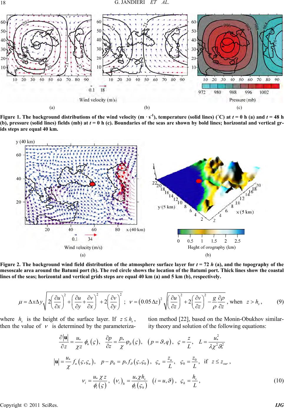

G. JANDIERI ET AL.
18
(a) (b) (c)
Figure 1. The background distributions of the wind veloc ity (m · s-1), temperature (solid lines) (˚C) at t = 0 h (a) and t = 48 h
(b), pressure (solid lines) fields (mb) at t = 0 h (c). Boundaries of the seas are show n by bold lines; horizontal and vertical gr-
ids steps are equal 40 km.
(a) (b)
Figure 2. The background wind field distribution of the atmosphere surface layer for t = 72 h (a), and the topography of the
mesoscale area around the Batumi port (b). The red circle show s the location of the Batumi por t. Thick lines show the coastal
lines of the seas; horizontal and vertical grids steps are equal 40 km (a) and 5 km (b), respectively.
22
2
22
uuv v
xy
x
yx y

  

 


 

;

22
2
0.05 2
uvg
zzzz




 
 
 


 , when
s
zh, (9)
where
s
h is the height of the surface layer. If
s
zh

,
then the value of

is determined by the parameteriza-tion method [22], based on the Monin-Obukhov similar- ity theory and solution of the following equations:

*,
u
u
zz




u

*,
p p
z








,pq  , ,
z
L
  2
*
22
*
u
L




*,,
uu
uf



u


0* 0
,pp pf


  , ,
u
u
z
L
  0
0,
z
L
  if
s
ur
zz,

*
ii
uz



,
 
*
s
ihih
uh






,iu

,
s
h
h
L


, (1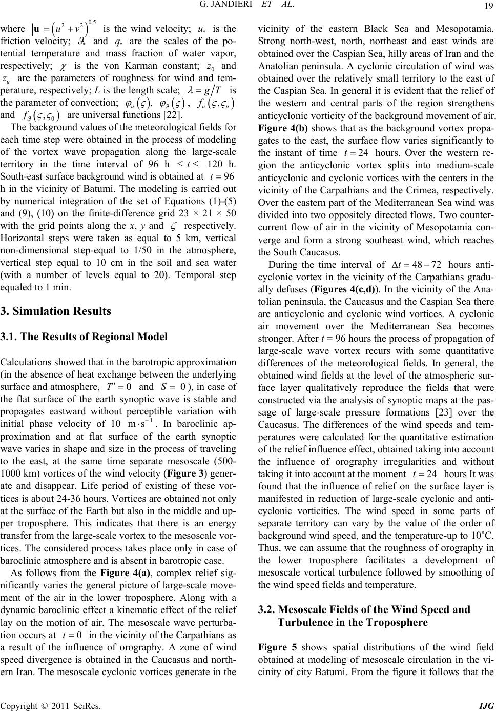0)

G. JANDIERI ET AL.
19
where

0.5
22
uvu is the wind velocity; * u is the
friction velocity; *

and * q are the scales of the po-
tential temperature and mass fraction of water vapor,
respectively;

is the von Karman constant; 0 z and
u
z are the parameters of roughness for wind and tem-
perature, respectively; L is the length scale;
g
T   is
the parameter of convection;

u

 ,




 ,


,
uu
f


and

0
,f


 are universal functions [22].
The background values of the meteorological fields for
each time step were obtained in the process of modeling
of the vortex wave propagation along the large-scale
territory in the time interval of 96 h t 120 h.
South-east surface background wind is obtained at 96t

h in the vicinity of Batumi. The modeling is carried out
by numerical integration of the set of Equations (1)-(5)
and (9), (10) on the finite-difference grid 23 × 21 × 50
with the grid points along the x, y and

respectively.
Horizontal steps were taken as equal to 5 km, vertical
non-dimensional step-equal to 1/50 in the atmosphere,
vertical step equal to 10 cm in the soil and sea water
(with a number of levels equal to 20). Temporal step
equaled to 1 min.
3. Simulation Results
3.1. The Results of Regional Model
Calculations showed that in the barotropic approximation
(in the absence of heat exchange between the underlying
surface and atmosphere, 0T and 0S), in case of
the flat surface of the earth synoptic wave is stable and
propagates eastward without perceptible variation with
initial phase velocity of 10 1
ms

. In baroclinic ap-
proximation and at flat surface of the earth synoptic
wave varies in shape and size in the process of traveling
to the east, at the same time separate mesoscale (500-
1000 km) vor tices of the wind v elocity ( Figure 3) gener-
ate and disappear. Life period of existing of these vor-
tices is about 24-36 hours. Vortices are obtained not only
at the surface of the Earth but also in the middle and up-
per troposphere. This indicates that there is an energy
transfer from the large-scale vortex to the mesoscale vor-
tices. The considered process takes place only in case of
baroclinic atmosphere and is absent in barotropic case.
As follows from the Figure 4(a), complex relief sig-
nificantly varies the general picture of large-scale move-
ment of the air in the lower troposphere. Along with a
dynamic baroclinic effect a kinematic effect of the relief
lay on the motion of air. The mesoscale wave perturba-
tion occurs at 0t in the vicinity of the Carpathians as
a result of the influence of orography. A zone of wind
speed divergence is obtained in the Caucasus and north-
ern Iran. The mesoscale cyclonic vortices generate in the
vicinity of the eastern Black Sea and Mesopotamia.
Strong north-west, north, northeast and east winds are
obtained over the Caspian Sea, hilly areas of Iran and the
Anatolian peninsula. A cyclonic circulation of wind was
obtained over the relatively small territory to the east of
the Caspian Sea. In general it is evident that the relief of
the western and central parts of the region strengthens
anticyclonic vorticity of th e background mov ement of air.
Figure 4(b) shows that as the background vortex propa-
gates to the east, the surface flow varies significantly to
the instant of time 24t

hours. Over the western re-
gion the anticyclonic vortex splits into medium-scale
anticyclonic and cyclonic vortices with the centers in the
vicinity of the Carpathians and the Crimea, respectively.
Over the eastern part of the Mediterranean Sea wind was
divided into two oppositely directed flows. Two counter-
current flow of air in the vicinity of Mesopotamia con-
verge and form a strong southeast wind, which reaches
the South Caucasus.
During the time interval of 48 72t hours anti-
cyclonic vortex in the vicinity of the Carpathians gradu-
ally defuses (Figures 4(с,d)). In the vicinity of the Ana-
tolian peninsula, the Caucasus and the Caspian Sea there
are anticyclonic and cyclonic wind vortices. A cyclonic
air movement over the Mediterranean Sea becomes
stronger. After t = 96 hours the process of propagation of
large-scale wave vortex recurs with some quantitative
differences of the meteorological fields. In general, the
obtained wind fields at the level of the atmospheric sur-
face layer qualitatively reproduce the fields that were
constructed via the analysis of synoptic maps at the pas-
sage of large-scale pressure formations [23] over the
Caucasus. The differences of the wind speeds and tem-
peratures were calculated for the quantitative estimation
of the relief influence effect, obtained taking into account
the influence of orography irregularities and without
taking it into account at the moment 24t hours It was
found that the influence of relief on the surface layer is
manifested in reduction of large-scale cyclonic and anti-
cyclonic vorticities. The wind speed in some parts of
separate territory can vary by the value of the order of
background wind speed, and th e temperature-up to 10˚C.
Thus, we can assume that the roughness of orography in
the lower troposphere facilitates a development of
mesoscale vortical turbulence followed by smoothing of
the wind speed fields and temperature.
3.2. Mesoscale Fields of the Wind Speed and
Turbulence in the Troposphere
Figure 5 shows spatial distributions of the wind field
obtained at modeling of mesoscale circulation in the vi-
cinity of city Batumi. From the figure it follows that the

G. JANDIERI ET AL.
20
Figure 3. The surface wind fields in the baroclyne approximation for a flat relief calculated at t = 0 h (a), 24 h (b), 48 h (c), 72
h (d), 96 h (e), and 120 h (f), respectively. Horizontal and vertical grids steps are equal 40 km.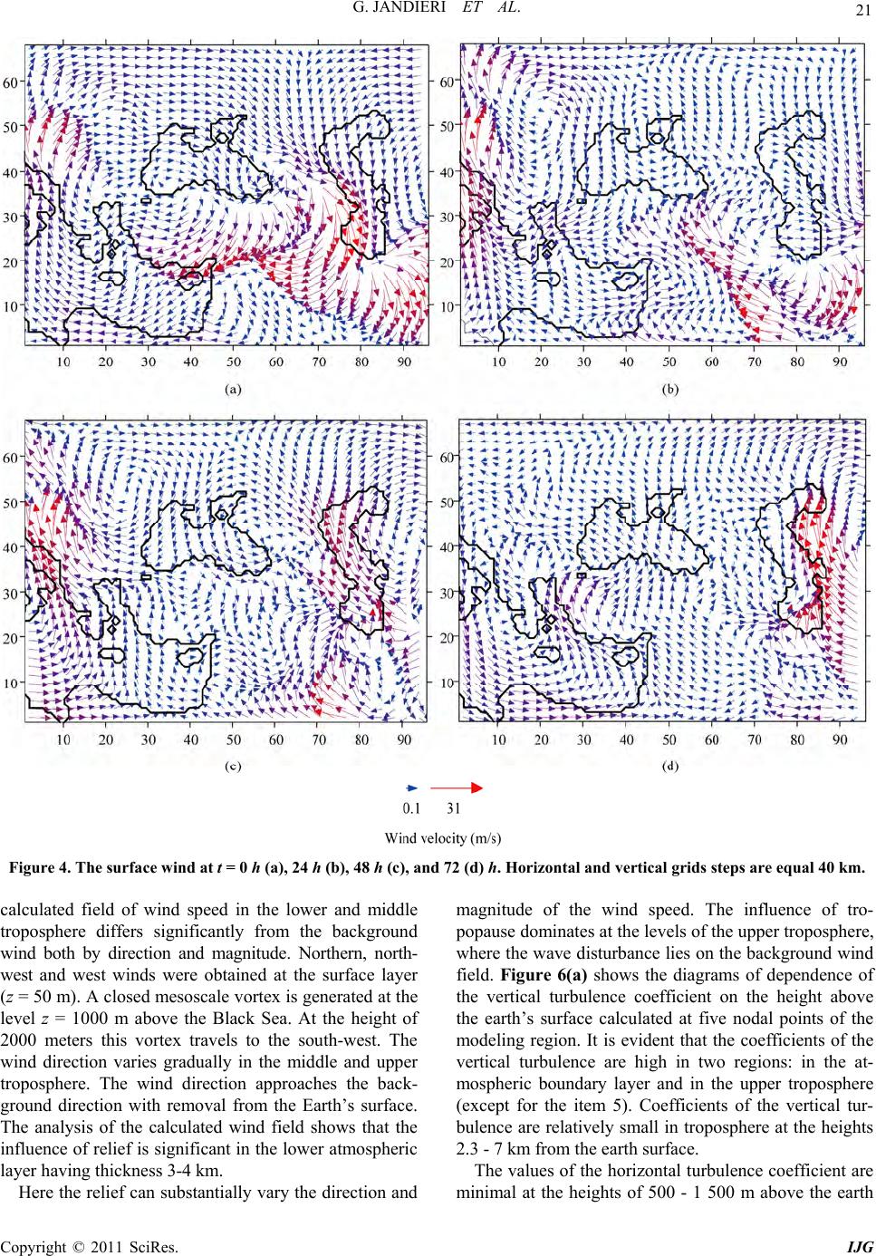

G. JANDIERI ET AL.
21
Figure 4. The surface wind at t = 0 h (a), 24 h (b), 48 h (c), and 72 (d) h. Horizontal and vertical grids steps are equal 40 km.
calculated field of wind speed in the lower and middle
troposphere differs significantly from the background
wind both by direction and magnitude. Northern, north-
west and west winds were obtained at the surface layer
(z = 50 m). A closed mesoscale vortex is generated at the
level z = 1000 m above the Black Sea. At the height of
2000 meters this vortex travels to the south-west. The
wind direction varies gradually in the middle and upper
troposphere. The wind direction approaches the back-
ground direction with removal from the Earth’s surface.
The analysis of the calculated wind field shows that the
influence of relief is significant in the lower atmospheric
layer having thickness 3-4 km.
Here the relief can substantially vary the direction and
magnitude of the wind speed. The influence of tro-
popause dominates at the levels of the upper troposphere,
where the wave disturbance lies on the background wind
field. Figure 6(a) shows the diagrams of dependence of
the vertical turbulence coefficient on the height above
the earth’s surface calculated at five nodal points of the
modeling region. It is evident that the coefficients of the
vertical turbulence are high in two regions: in the at-
mospheric boundary layer and in the upper troposphere
(except for the item 5). Coefficients of the vertical tur-
bulence are relatively small in troposphere at the heights
2.3 - 7 km from the earth surface.
The values of the horizontal turbulence coefficient are
minimal at the heights of 500 - 1 500 m above the earth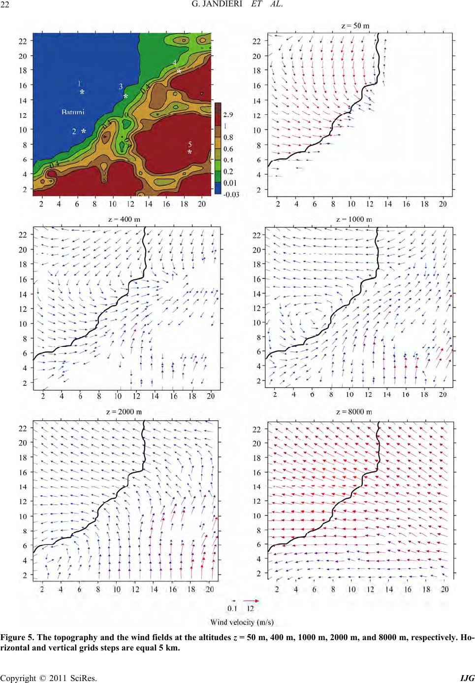

G. JANDIERI ET AL.
22
Figure 5. The topography and the wind fie lds at the altitudes z = 50 m, 400 m, 1000 m, 2000 m, and 8000 m, respectively. Ho-
rizontal and vertical grids steps are equal 5 km.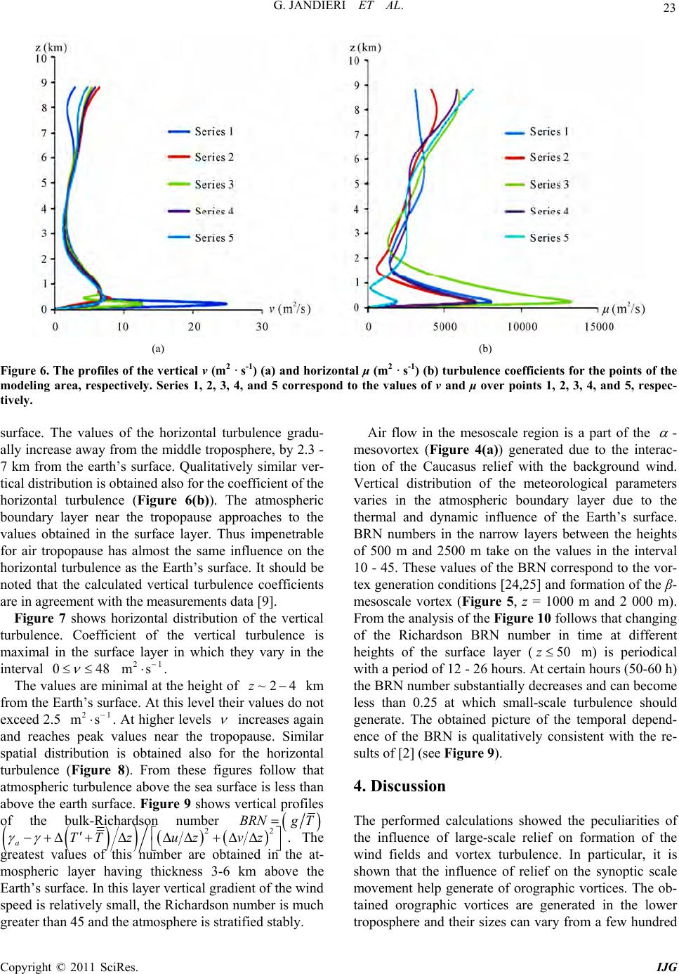

G. JANDIERI ET AL.
23
(a) (b)
Figure 6. The profiles of the vertical ν (m2 · s-1) (a) and horizontal μ (m2 · s-1) (b) turbulence coefficients for the points of the
modeling area, respectively. Series 1, 2, 3, 4, and 5 correspond to the values of ν and μ over points 1, 2, 3, 4, and 5, respec-
tively.
surface. The values of the horizontal turbulence gradu-
ally increase away from the middle troposphere, by 2.3 -
7 km from the earth’s surface. Qualitatively similar ver-
tical distribution is obtained also for the coefficient of the
horizontal turbulence (Figure 6(b)). The atmospheric
boundary layer near the tropopause approaches to the
values obtained in the surface layer. Thus impenetrable
for air tropopause has almost the same influence on the
horizontal turbulence as the Earth’s surface. It should be
noted that the calculated vertical turbulence coefficients
are in agreement with the measurements data [9].
Figure 7 shows horizontal distribution of the vertical
turbulence. Coefficient of the vertical turbulence is
maximal in the surface layer in which they vary in the
interval 048

 21 ms

.
The values are minimal at the height of ~2 4z

km
from the Earth’s surface. At this level their values do not
exceed 2.5 21 ms

. At higher levels

increases again
and reaches peak values near the tropopause. Similar
spatial distribution is obtained also for the horizontal
turbulence (Figure 8). From these figures follow that
atmospheric turbulence above the sea surface is less than
above the earth surface. Figure 9 shows vertical profiles
of the bulk-Richardson number


BRNg T
 

22
aTT zuzvz



 

. The
greatest values of this number are obtained in the at-
mospheric layer having thickness 3-6 km above the
Earth’s surface. In this layer vertical gr adient of the wind
speed is relatively small, the Richardson number is much
greater than 45 and the atmosphere is stratified stably.
Air flow in the mesoscale region is a part of the

-
mesovortex (Figure 4(a)) generated due to the interac-
tion of the Caucasus relief with the background wind.
Vertical distribution of the meteorological parameters
varies in the atmospheric boundary layer due to the
thermal and dynamic influence of the Earth’s surface.
BRN numbers in the narrow layers between the heights
of 500 m and 2500 m take on the values in the interval
10 - 45. These values of the BRN correspond to the vor-
tex generation conditions [24,25] and formation of the β-
mesoscale vortex (Figure 5, z = 1000 m and 2 000 m).
From the analysis of the Figure 10 follows that changing
of the Richardson BRN number in time at different
heights of the surface layer (50z m) is periodical
with a period of 12 - 26 hours. At cer tain hours (50 -60 h)
the BRN number substantially decreases and can become
less than 0.25 at which small-scale turbulence should
generate. The obtained picture of the temporal depend-
ence of the BRN is qualitatively consistent with the re-
sults of [2] (see Figure 9).
4. Discussion
The performed calculations showed the peculiarities of
the influence of large-scale relief on formation of the
wind fields and vortex turbulence. In particular, it is
shown that the influence of relief on the synoptic scale
movement help generate of orographic vortices. The ob-
tained orographic vortices are generated in the lower
troposphere and their sizes can vary from a few hundred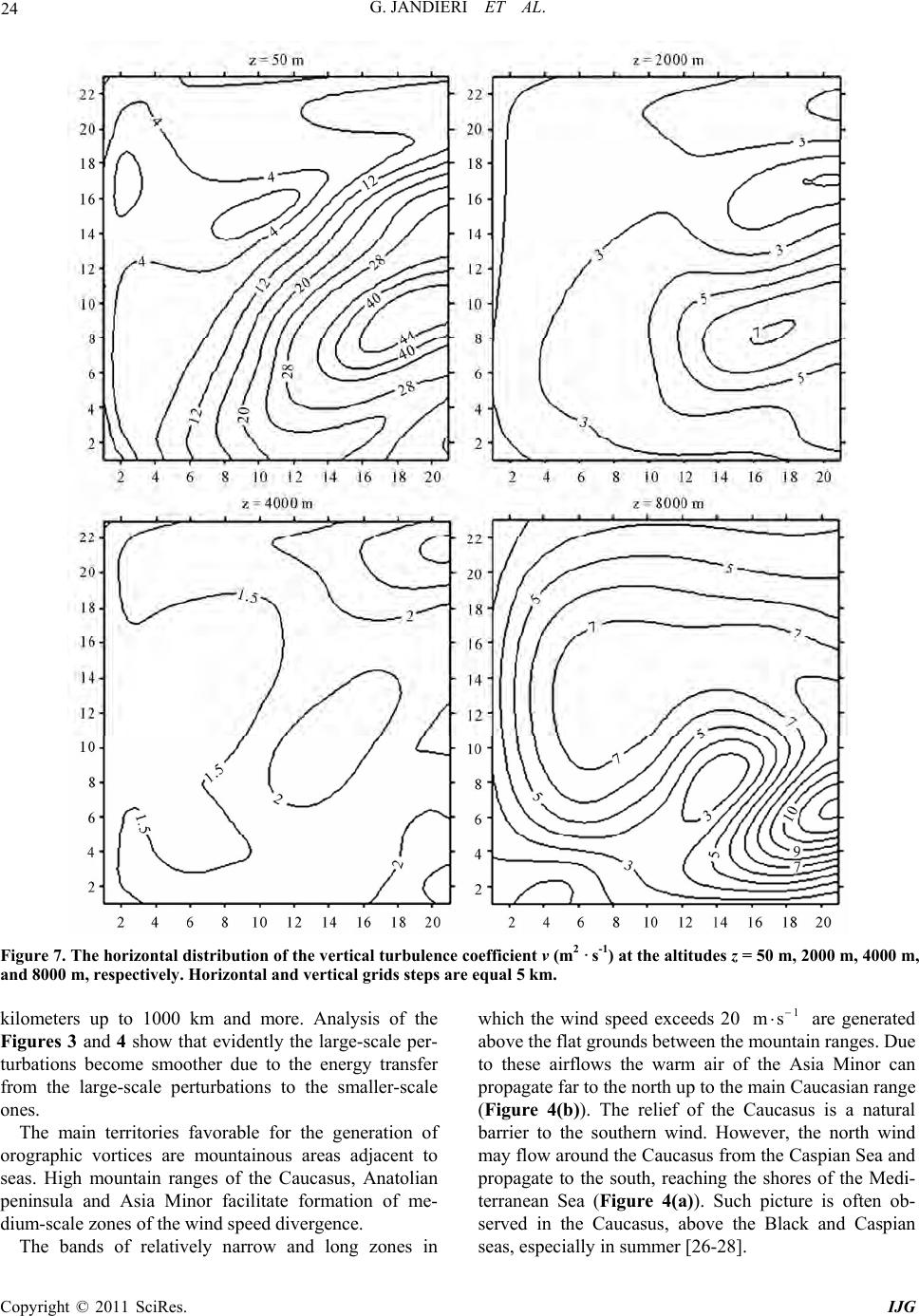

G. JANDIERI ET AL.
24
Figure 7. The horizontal distribution of the vertical turbulence coefficient ν (m2 · s-1) at the altitudes z = 50 m, 2000 m, 4000 m,
and 8000 m, respectively. Horizontal and vertical grids steps are equal 5 km.
kilometers up to 1000 km and more. Analysis of the
Figures 3 and 4 show that evidently the large-scale per-
turbations become smoother due to the energy transfer
from the large-scale perturbations to the smaller-scale
ones.
The main territories favorable for the generation of
orographic vortices are mountainous areas adjacent to
seas. High mountain ranges of the Caucasus, Anatolian
peninsula and Asia Minor facilitate formation of me-
dium-scale zones of the wind speed divergence.
The bands of relatively narrow and long zones in
which the wind speed exceeds 20 1 ms

 are generated
above the flat grounds between the mountain ranges. Due
to these airflows the warm air of the Asia Minor can
propagate far to the north up to the main Caucasian range
(Figure 4(b)). The relief of the Caucasus is a natural
barrier to the southern wind. However, the north wind
may flow around the Caucasus from the Caspian Sea and
propagate to the south, reaching the shores of the Medi-
terranean Sea (Figure 4(a)). Such picture is often ob-
served in the Caucasus, above the Black and Caspian
seas, especially in summer [26-28].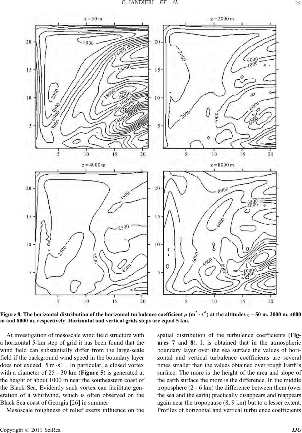

G. JANDIERI ET AL.
25
Figure 8. The horizontal distribution of the horizontal turbulence coefficient μ (m2 · s-1) at the altitudes z = 50 m, 2000 m, 4000
m and 8000 m, respectively. Horizontal and vertical grids steps are equal 5 km.
At investigation of mesoscale wind field structure with
a horizontal 5-km step of grid it has been found that the
wind field can substantially differ from the large-scale
field if the back ground wind speed in the boundar y layer
does not exceed 1 5m s

. In particular, a closed vortex
with a diameter of 25 - 30 km (Figure 5) is generated at
the height of abou t 1000 m near the southe astern coast of
the Black Sea. Evidently such vortex can facilitate gen-
eration of a whirlwind, which is often observed on the
Black Sea coast of Georgia [26] in summer.
Mesoscale roughness of relief exerts influence on the
spatial distribution of the turbulence coefficients (Fig-
ures 7 and 8). It is obtained that in the atmospheric
boundary layer over the sea surface the values of hori-
zontal and vertical turbulence coefficients are several
times smaller than the values obtained over rough Earth’s
surface. The more is the height of the area and slope of
the earth surface the more is the difference. In the middle
troposphere (2 - 6 km) the difference between them (over
the sea and the earth) practically disappears and reappears
again near the tropopause (8, 9 km) but to a lesser extent.
Profiles of horizontal and vertical turbulence coefficients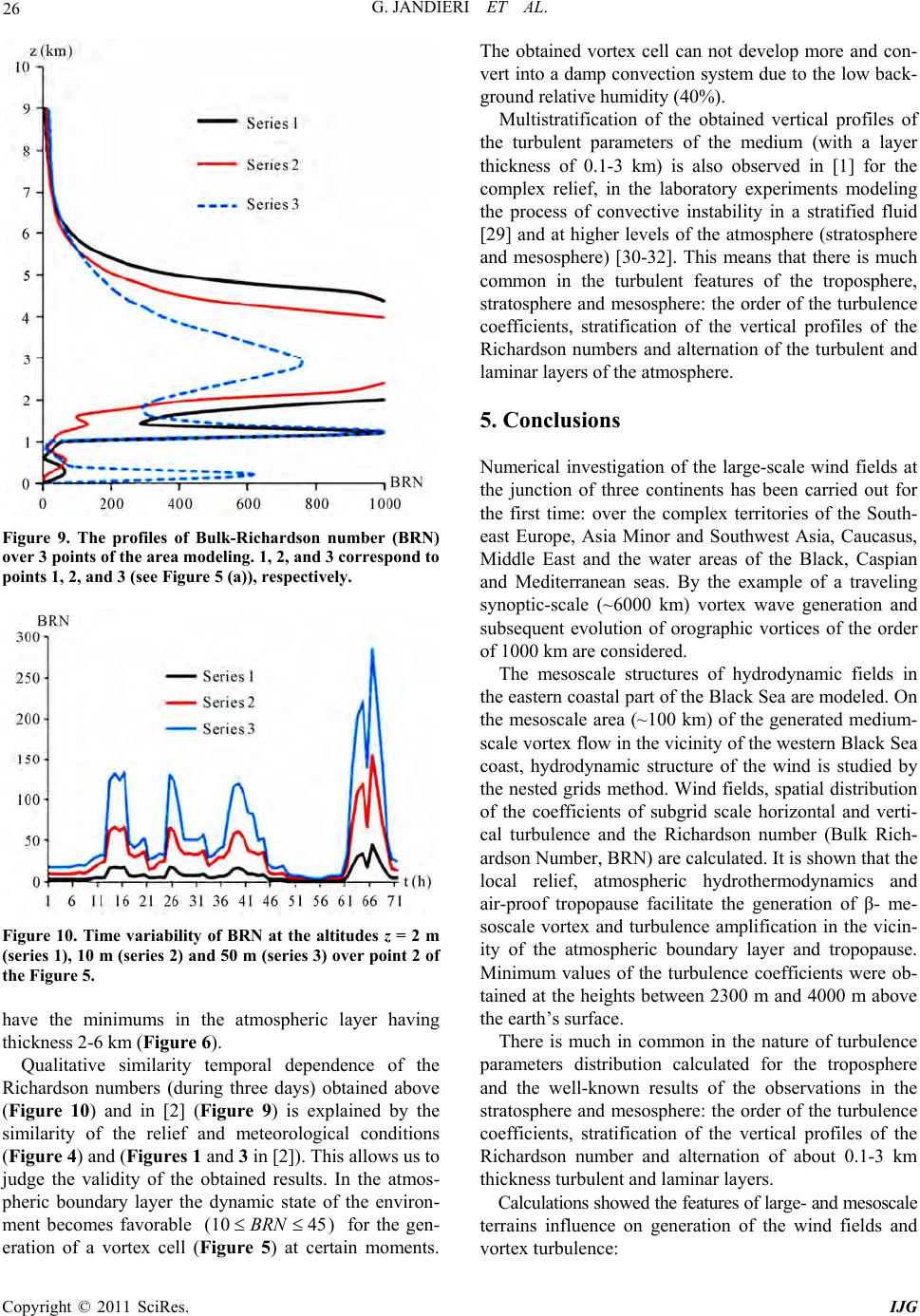

G. JANDIERI ET AL.
26
Figure 9. The profiles of Bulk-Richardson number (BRN)
over 3 points of the area modeling. 1, 2, and 3 correspond to
points 1, 2, and 3 (see Figure 5 (a)), respectively.
Figure 10. Time variability of BRN at the altitudes z = 2 m
(series 1), 10 m (series 2) and 50 m (series 3) over point 2 of
the Figure 5.
have the minimums in the atmospheric layer having
thickness 2 -6 km (Figure 6).
Qualitative similarity temporal dependence of the
Richardson numbers (during three days) obtained above
(Figure 10) and in [2] (Figure 9) is explained by the
similarity of the relief and meteorological conditions
(Figure 4) and (Figures 1 and 3 in [2]). This allows us to
judge the validity of the obtained results. In the atmos-
pheric boundary layer the dynamic state of the environ-
ment becomes favorable (10 45)BRN

 for the gen-
eration of a vortex cell (Figure 5) at certain moments.
The obtained vortex cell can not develop more and con-
vert into a damp convection system due to the low back-
ground relative humidity (40%).
Multistratification of the obtained vertical profiles of
the turbulent parameters of the medium (with a layer
thickness of 0.1-3 km) is also observed in [1] for the
complex relief, in the laboratory experiments modeling
the process of convective instability in a stratified fluid
[29] and at higher levels of the atmosphere (stratosphere
and mesosphere) [30-32]. This means that there is much
common in the turbulent features of the troposphere,
stratosphere and mesosphere: the order of the turbulence
coefficients, stratification of the vertical profiles of the
Richardson numbers and alternation of the turbulent and
laminar layers of the atmosphere.
5. Conclusions
Numerical investigation of the large-scale wind fields at
the junction of three continents has been carried out for
the first time: over the complex territories of the South-
east Europe, Asia Minor and Southwest Asia, Caucasus,
Middle East and the water areas of the Black, Caspian
and Mediterranean seas. By the example of a traveling
synoptic-scale (~6000 km) vortex wave generation and
subsequent evolution of orographic vortices of the order
of 1000 km are considered.
The mesoscale structures of hydrodynamic fields in
the eastern coastal part of the Black Sea are modeled. On
the mesoscale area (~100 km) of the generated medium-
scale vortex flow in the vicinity of the western Black Sea
coast, hydrodynamic structure of the wind is studied by
the nested grids method. Wind fields, spatial distribution
of the coefficients of subgrid scale horizontal and verti-
cal turbulence and the Richardson number (Bulk Rich-
ardson Number, BRN) are calculated. It is shown that the
local relief, atmospheric hydrothermodynamics and
air-proof tropopause facilitate the generation of β- me-
soscale vortex and turbulence amplification in the vicin-
ity of the atmospheric boundary layer and tropopause.
Minimum values of the turbulence coefficients were ob-
tained at the heights between 2300 m and 4000 m above
the earth’s surface.
There is much in common in the nature of turbulence
parameters distribution calculated for the troposphere
and the well-known results of the observations in the
stratosphere and mesosphere: the order of the turbulence
coefficients, stratification of the vertical profiles of the
Richardson number and alternation of about 0.1-3 km
thickness turbulent and laminar layers.
Calculations showed the features of large- and mesoscale
terrains influence on generation of the wind fields and
vortex turbulence:

G. JANDIERI ET AL.
27
 Large and high mountain ranges of the Caucasus,
Minor and Southwest Asia facilitate formation of
medium-scale zones of wind speed divergence and
vortex structures;
 The main favorable territories for the generation of
orographic vortices are the neighborhoods of the
Carpathian Mountains and the Black, Caspian and
Mediterranean seas;
 The orographic vortices are generated in the lower
troposphere and their sizes can vary from a few
hundred kilometers to 1 thousand kilometers and
higher;
 Atmosphere tends to a smoother distribution of the
large-scale meteorological fields due to the oro-
graphic vortices;
 Separate β-mesoscale vortices can generate against
the background of the α-mesoscale vortices in the
atmospheric boundary layer in the vicinity of the
sea-land at the low values of the vertical wind
speed gradients;
 The underlying surface and impenetrability of tro-
popause equally facilitate turbulence amplification
of the atmosphere;
 There are 0.1-3 km thickness turbulent stratifica-
tions in the troposphere similar as in 10 km layers
of stratosphere and middle atmosphere;
 Vertical profiles of the Richardson numbers and
the turbulence coefficients contain several (3-5)
extremums.
The objective of the further investigation is specifica-
tion of the atmosphere turbulization mechanisms, gen-
eration and evolution of the vortex structures over the
considered complex terrain in the large and mesoscale
hydrodynamic processes.
6. References
[1] A. P. Weigel, F. K. Chow and M. W. Rotach, “On the
Nature of Turbulent Kinetic Energy in a Steep and Nar-
row Alpine Valley,” Boundary-Layer Meteorology
Springer Science-Business Media B.V., Vol. 123, 2006,
pp. 177-199. doi:10.1007/s10546-006-9142-9
[2] S. Kirkwood, M. Mihalikova, T. N. Rao and K. Satheesan,
“Turbulence Associated with Mountain Waves over
Northern Scandinavia–a Case Study Using the ESRAD
VHF Radar and the WRF Mesoscale Model,” Atmos-
pheric Chemistry and Physics Discussions, Vol. 9, No. 5,
2009, pp. 20775-20817. doi:10.5194/acpd-9-20775-2009
[3] G. D. Nastrom, K. S. Gage and W. L. Ecklund, “Variabil-
ity of Turbulence, 4 - 20 km, in Colorado and Alaska
from MST Radar Observations,” Journal of Geophysical
Research, Vol. 91, 1986, pp. 6722-6734.
doi:10.1029/JD091iD06p06722
[4] W. K. Hocking and J. Röttger, “The Structure of Turbu-
lence in the Middle and Lower Atmosphere Seen by and
Deduced from MF, HF and VHF Radar, with Special
Emphasis on Small-Scale Features and Anisotropy,” An-
nales Geophysicae, Vol. 19, 2001, pp. 933-944.
doi:10.5194/angeo-19-933-2001
[5] W. D. Smyth and W. R. Peltier, “The Transition between
Kelvin-Helmholtz and Holmboe Instability: An Investi-
gation of the Over-Reflection Hypothesis,” Journal of the
Atmospheric Sciences, Vol. 46, No. 24, 1989, pp. 3698-
3720.
doi:10.1175/1520-0469(1989)046<3698:TTBKAH>2.0.C
O;2
[6] P. W. Chan, “Determination of Richardson number Pro-
file from Remote Sensing Data and Its Aviation Applica-
tion,” Proceedings 14th International Symposium for the
Advancement of Boundary Layer Remote Sensing, IOP
Conf. Series: Earth and Environmental Science 1, 012043,
2008. doi:10.1088/1755-1307/1/1/012043
[7] Yu. Zhao, X. P. Cui and S. Gao, “Richardson Number in
a Moist Atrmosphere and Its Application in the Analysis
of Heavy Rainfall Events,” Acta Meteorologica Sinica,
Vol. 24, 2010, No 1, pp. 95-103.
[8] C. G. Lu and S. E. Koch, “Interaction of Upper-Tropo-
spheric Turbulence and Gravity Waves Obtaned from
Spectral Structure Function Analyses,” Journal of the
Atmospheric Sciences, Vol. 65, No. 8, 2008, pp. 2676-
2690.
doi:10.1175/2007JAS2660.1
[9] N. M. Gavrilov and I. S. Fukao, “Numerical and the MU
Radar Estimations of Gravity Wave Enhancement and
Turbulent Ozone Fluxes Near the Tropopause,” Annales
Geophysicae, Vol. 22, No. 11, 2004, pp. 3889-3898 and p.
SRef-ID: 1432-0576/ag/2004-22-3889.
[10] G. Dutta, M. C. A. Kumar, P. V. Kumar, P. V. Rao, B.
Bapiraju and H. A. Basha, “High Resolution Observa-
tions of Turbulence in the Troposphere and Lower
Stratosphere over Gadanki,” Annales Geophysicae, Vol.
27, No. 6, 2009, pp. 2407-2415.
doi:10.5194/angeo-27-2407-2009
[11] A. A. Kordzadze, A. A. Surmava, D. I. Demetrashvili,
and V. G. Kukhalashvili, “Numerical Investigation of the
Influence of the Caucasus Relief on the Distribution of
Hydrometeorological Fields,” Izvestia, Atmospheric and
Oceanic Physics, Vol. 43, No. 6, 2007, pp. 783-791.
doi:10.1134/S0001433807060060
[12] G. I. Marchuk, “The Numerical Solution of the Problems
of Dynamics of the Atmosphere and Ocean,” Hydrome-
teoizdat, Leningrad, 1974 (in Russian).
[13] L. N. Gutman, “Introduction to the Nonlinear Theory of
Mesometeorological Processes in the Atmosphere,” Hy-
drometeoizdat, Leningrad, 1969 (In Russian).
[14] L. T. Matveev, “The Course of General Meteorology,
Physics of Atmosphere and Ocean,” Hydrometeoizdat,
Leningrad, 1984 (In Russian).
[15] A. F. Chudnovski, “Heat Physics of Soils,” Nauka, Mos-
cow, 1976 (In Russian).
[16] G. I. Marchuk, V. P. Dimnikov, V. B. Zalesnii, V. N.
Likosov and V. Ya. Galin, “The Mathematical Simulation
of General Circulation of the Atmosphere and Ocean,”

G. JANDIERI ET AL.
28
Hydrometeoizdat, Leningrad, 1984 (In Russian).
[17] P. N. Belov, E. P. Borisenkov and B. D. Panin, “The
Numerical Methods of Weather Forecast,” Hydrometeo-
izdat, Leningrad, 1989 (In Russian).
[18] F. G. Shuman and L. R. Hovermale, “An Operational
Six-Layer Primitive Equation Model,” Journal of Applied
Mechanics, Vol. 7, No. 4, 1968, pp. 525-547.
[19] E. Palmen and C. W. Newton, “Atmospheric Circulation
Systems”. Academic Press, New York and London, 1969.
[20] S. S. Zilitinkevich and A. S. Monin, “The Turbulence in
Dynamical Models of the Atmosphere,” Nauka, Lenin-
grad, 1971.
[21] G. I. Marchuk, V. P. Kochergin, A. S. Sarkisyan et al.,
“Mathematical Models of Ocean Circulation,” Nauka,
Novosibirsk, 1980.
[22] A. L. Kazakov and G. L. Lazriev, “About Parameteriza-
tion of the Surface Layer of the Atmosphere and Active
Layer of the Soil,” Izvestia AN SSSR, Phizika Atmosfery i
Okeana, Vol. 14, No. 3, 1978, pp. 257-265.
[23] K. I. Papinashvili, “Atmospheric Processes in Transcau-
casia and Their Relation with Macrocirculation Processes
Above the Territory of Eurasia,” Hydrometeoizdat, Len-
ingrad, 1963, p. 184.
[24] T. W. Troutman, D. B. Elson and M. A. Rose, “A Severe
Weather Threads Checklist to Determine Pre-Storm En-
vironment,” www.srh.noaa.gov/ohx/?n=checklist
[25] “Bulk Richardson Number,” Wikipedia, the free ency-
clopedia.
http://www.mythical-buddies.com/index.php?q=Bulk_Ri
chardson_number
[26] M. Kordzakhia, “The Climate of Georgia,” Publishing
House of the Georgian Academy of Sciences, Tbilisi,
1961.
[27] “The Atlas of Excitement and a Wind of the Black Sea,”
Gidrometeoizdat, Leningrad, 1969.
[28] “The Climate and Climatic Resources of Georgia,”
Gidrometeoizdat, Leningrad, 1971.
[29] Yu. D. Chashechkin, “Stochasticity of Convective Flows
in a Stratified Liquid. Non-Linear Waves: Stochasticity
and Turbulence,” Gorky: AN SSSR, IPF, 1980, pp. 131-
139.
[30] E. V. Thrane et al., “Neutral Air Turbulence in the Upper
Atmosphere Observed during the Energy Budget Cam-
paign,” Journal of Atmosphere and Terrestrial Physics,
Vol. 47, No. 1, 1985, pp. 243-264.
doi:10.1016/0021-9169(85)90136-9
[31] F. J. Schmidlin, M. Carlson, D. Rees, D. Offermann,
Philbrick and H. U. Widdel, “Wind Structure and Vari-
ability in the Middle Atmosphere during the November
1980 Energy Budget Campaign,” Journal of Atmosphere
and Terrestrial Physics, Vol. 47, 1985, pp. 183-193.
doi:10.1016/0021-9169(85)90133-3
[32] A. I. Gvelesiani and A. T. Eliava, “On the Subrange of
Buoyancy of the Turbulent Mesosphere,” Izv. RAN, FAO,
Vol. 34, No. 2, 1998, pp. 241-244.