 American Journal of Operations Research, 2013, 3, 521-535 Published Online November 2013 (http://www.scirp.org/journal/ajor) http://dx.doi.org/10.4236/ajor.2013.36051 Open Access AJOR Models for Ordering Multiple Products Subject to Multiple Constraints, Quantity and Freight Discounts John Moussourakis, Cengiz Haksever Department of Information Systems and Supply Chain Management, College of Business Administration, Rider University, Lawrenceville, USA Email: haksever@rider.edu Received August 5, 2013; revised September 5, 2013; accepted September 13, 2013 Copyright © 2013 John Moussourakis, Cengiz Haksever. This is an open access article distributed under the Creative Commons Attri- bution License, which permits unrestricted use, distribution, and reproduction in any medium, provided the original work is properly cited. ABSTRACT One of the most important responsibilities of a supply chain manager is to decide “how much” (or “many”) of inventory items to order and how to transport them. This paper presents four mixed-integer linear programming models to help supply chain managers make these decisions for multiple products subject to multiple constraints when suppliers offer quantity discounts and shippers offer freight discounts. Each model deals with one of the possible combinations of all-units, incremental quantity discounts, all-weight and incremental freight discounts. The models are based on a piecewise linear approximation of the number of orders function. They allow any number of linear constraints and de- termine if independent or common (fixed) cycle ordering has a lower total cost. Results of computational experiments on an example problem are also presented. Keywords: Inventory; Mixed-Integer Linear Programming; Quantity and Freight Discounts; All-Units and Incremental Discounts; Multiple Products and Multiple Constraints 1. Introduction Supply chain management has been receiving an ever- increasing attention from both academicians and business managers for the past several decades. The main reason for this attention seems to be the realization that a well coordinated supply chain will lead to lower costs, and hence greater profits, for its members compared to the costs incurred by members of a supply chain that is not coordinated. Two of the major cost components in a supply chain are inventory and transportation costs. According to 2013 Annual State of Logistics Report [1] of Council of Sup- ply Chain Management Professionals (CSCMP), the av- erage investment in all business inventories (agriculture, mining, construction, services, manufacturing, wholesale, and retail trade) reached to almost $2.3 trillion in 2012, which was equivalent to 8.5 percent of the Gross Domes- tic Product (GDP) of the same year. In this total there are inventory carrying costs and transportation (all modes) costs, $434 billion and $897 billion, respectively. One of the conclusions of the report was: “Record high invento- ries could become a drag on the economy if we do not start drawing them down.” Clearly, managing and re- ducing these costs will not only help the economy but also reduce the operating costs of any company and boost its profits. The importance of inventory carrying costs and trans- portation costs has been well understood and appreciated by the operations research community as evidenced by the extensive list of publications on the optimization of inventory and transportation decisions. This paper aims to make a contribution to an area of this rich field of re- search that has not seen much development. Specifically, this paper presents a zero-one mixed-in- teger linear programming model for the optimization of lot-sizing decisions for buyers ordering multiple products subject to multiple linear constraints when they are of- fered quantity (price) discounts by suppliers and freight discounts by shippers. The model provides an approxi- mate optimal solution based on a linear approximation of the number of orders function, which can be achieved as closely as the analyst desires. This paper is an extension of our earlier research [2]. While published models deal with small number of constraints and either fixed (com- mon) or independent cycle solutions, the proposed mod-  J. MOUSSOURAKIS, C. HAKSEVER Open Access AJOR 522 els may include any number of linear constraints and determine which of the two cycle types leads to a lower total cost. Finally, we present models that, when avail- able, take advantage of quantity discounts and freight discounts of both kinds (i.e., all-units and incremental). The paper is organized as follows: A survey of litera- ture is presented in the next section. The third section provides preliminaries. The fourth section presents vari- ables and parameters, and four mixed-integer linear pro- gramming models. Section five presents computer im- plementation and results of computational experiments. A summary and conclusions are given in section six. Two appendices provide relevant mathematical back- ground that forms the foundation for the four models. 2. Literature Review There is an extensive literature on quantity discount mo- dels. A comprehensive review of literature until 1995 can be found in Benton and Park [3] where papers dealing with both all-units and incremental quantity discounts are reviewed. Another review can be found in Munson and Rosenblatt [4]. The focus in this paper is on modeling lot-sizing decisions for multiple products subject to mul- tiple linear constraints when both quantity (i.e. unit price) and freight (i.e., unit shipment) discounts of both kinds (i.e., all-units and incremental) are available to a buyer. Therefore, we limit our review to a narrow portion of the literature. 2.1. Single Product, Quantity and Freight Discounts, Unconstrained Case Tersine and Barman [5] derived lot-sizing optimization algorithms for quantity and freight discount situations for both all-units quantity discounts and all-weights freight discounts. These authors extended their algorithms to an incremental case in a separate paper [6]. Arcelus and Rowcroft [7] developed an all-units quantity and all- weight freight discounts model for lot-sizing decision with the possibility of disposal. Diaby and Martel [8] developed a mixed-integer linear programming model for optimal purchasing and shipping quantities in a multi- echelon distribution system with deterministic, time- varying demands. Tersine, Barman, and Toelle [9] pro- posed a composite model that included a variety of rele- vant inventory costs and developed algorithms for the optimization of lot-sizing decision where all-units or in- cremental quantity discounts and all-weight and incre- mental freight discounts were combined into a single res- tructured discount schedule. Burwell, et. al. [10] incur- porated all-units quantity and all-weight freight dis- counts in a lot sizing model when demand is dependent upon price. They developed an algorithm to determine the optimal lot size and selling price for a class of de- mand functions. Darwish [11] investigated the effects of transportation and purchase price in all combinations of all-units/incremental discounts and all-weight/incremental freight discounts for stochastic demand. Mendoza and Ventura [12] developed exact algorithms for deciding economic lot sizes under all-units and incremental quan- tity discounts and two modes of transportation: truck load and less than truck load. Toptal [13] developed a model for lot sizing decisions involving stepwise freight costs and all-units quantity discounts. 2.2. Multiple Products, All-Units and Incremental Quantity Discounts, Constrained Case None of the papers reviewed in this section incorporated both quantity and freight discounts; however, they dealt with multiple products and at most two constraints. Ben- ton [14] was the first to consider the problem for multiple products with budget and space constraints. In this paper, the author developed a heuristic procedure for order quan- tity when all-units quantity discounts were available from multiple suppliers. Rubin and Benton [15] considered the same problem as Benton [14] and presented a set of al- gorithms that collectively found the optimal order vec- tor. In a more recent paper, Rubin and Benton [16] ex- tended their solution methods to the same setup with in- cremental quantity discounts. Guder, et al. [17] presented a method for determining optimal order quantities subject to a single resource con- straint under incremental quantity discounts. The method involves the evaluation of every feasible price level combination for each item. The authors point out that due to the combinatorial nature of the method, it is impracti- cal for a large number of items; however, they offer a heuristic algorithm for large problems. To the best of our knowledge, there is no published model for ordering multiple products subject to more than two constraints when both quantity and freight discounts are available. 3. Preliminaries We assume an inventory system involving multiple products with known and constant independent demand, instantaneous replenishment, and constant lead times where no shortages are allowed. Without loss of general- ity we assume a zero lead time. Ordering cost for each product is a fixed amount that is independent of order size. Inventory holding (carrying) cost for each product is a percent of the purchase price, per unit per year; the same percentage applies to all products. In this paper four models are presented corresponding to all four combinations of quantity and freight discounts. For example, Model I has been developed to determine the optimal order quantity when all suppliers offer all-  J. MOUSSOURAKIS, C. HAKSEVER Open Access AJOR 523 units quantity discounts and all shippers offer all-units freight constraints. Model III is for a situation in which suppliers offer all-units price discounts while shippers offer incremental freight discounts. The decision maker’s objective is to minimize the total annual inventory hold- ing, ordering, and purchase cost subject to multiple linear constraints, such as a limit on total inventory investment at any time, warehouse space, volume, and/or weight, an upper limit on the number of orders, etc. The four models rely on the functional relationship between the number of orders and order quantity which enables us to handle multiple constraints and multiple price-breaks through a linear model. We develop a zero- one mixed-integer linear programming model based on the piece-wise approximation of the number of orders function of each product. The approximation can be car- ried to any finite degree of closeness. Let Xj = Order quantity, and Dj = Annual demand for product j. Then the number of orders function jjjj NfX DX is strictly convex (Figure 1) and can be approximated with a series of linear functions. Although the function is continuous everywhere for 1 ≤ Xj ≤ Dj, this interval has ej subintervals corresponding to discount intervals and therefore the number of orders curve has segments that correspond to these intervals. Considering any such segment of the curve, any line segment such as L = a bX, passing through the end points of the interval will always be above the curve and L will always overestimate the true number of orders in that interval. The error of estimation, E, will be given by ELNabX DX . The maximum error can be reduced to any finite num- ber by increasing the number of line segments. Once a decision maker chooses the maximum tolerable error (TE), the range of possible order sizes (Xj) is split into as many intervals as necessary so that no line segment overestimates N by more than TE. One way this number may be selected is by dividing the tolerable excess cost resulting from the overestimation of the true number of orders, by the sum of the ordering cost. We follow a procedure that splits an interval at the point (Xio) where the error E is maximum, thereby reducing overestimation by the greatest amount. The details of the linearization of the number of orders function are given in Appendix A. Suppliers frequently offer their products at lower prices to those who buy them in large quantities. In this system the supplier identifies intervals of possible order quanti- ties and a price for each interval, which is progressively Figure 1. Piecewise linear approximation of the number of orders function in the hth discount step, h = 1, 2,···, ej.  J. MOUSSOURAKIS, C. HAKSEVER Open Access AJOR 524 lower for higher quantity intervals. A quantity dis- count schedule for a product can be represented as follows: 11 1 22 2 for for for jj jj j jj j j ejej j PKXU PKXU P PKX where Pj is the price paid for product j, Phj is the price to be paid if the order quantity Xj falls in discount interval h, and Khj and Uhj’s are quantities that define discount in- tervals. Similarly, a freight discount schedule can be re- presented as: 111 222 for for for jj jj j jj j sj ejej j CKXU CKXU C CKX The most frequently encountered discount schedules are all-units and incremental. An all-units discount scheme assumes that the lowest price for which an order quantity qualifies will be paid for all the units purchased. In an incremental discount system the lowest price is paid only for the units in the relevant interval and higher prices for quantities in lower intervals. Next, decision variables and parameters of Model I are presented. 4. Models for Optimizing Lot-Sizing Decisions 4.1. Decision Variables Xhij = order quantity for product j in subinterval i of the price discount interval h, Xj = order quantity to be adopted for product j, hj = order quantity for product j in the shipping cost discount interval h, = order quantity for product j suggested from the shipping cost discount schedule, Nj = number of orders to be adopted for product j, POj = amount paid for order size Xj, product j (i.e., dollar amount paid for one order, excluding shipping and ordering costs), Pj = price to be paid for product j, Csj = shipping cost per unit paid for product j, Tj = cycle time for product j, Yhj = auxiliary variables for product j: Yhj = 1, if , ; 0 jhjhjhj XnmY , otherwise, auxiliaryvariablesforproduct: 1if, ;0,otherwise, hj hjjhj hjhj Yj YXnmY Yhij = auxiliary variables for product j: Yhij = 1, if , ; 0 jhij hijhij XnmY , otherwise, Lhij = number of orders if the order size is in subinter- val i of price discount interval h for product j, hij L number of orders if the order size is in subin- terval i of freight discount interval h for product j. 4.2. Model Parameters TC = total annual inventory cost, k = number of products, Coj = ordering cost for product j, 1, 2,,jk, Ccj = holding (carrying) cost per unit per year for pro- duct j, Cshj = shipping cost per unit if the order quantity falls in the shipping cost discount interval h, 1, 2,,j he , I = percent of average price as holding cost, Phj = price to be paid if the order quantity Xj falls in price discount interval h, 1, 2,,j he, ej = number of price discount intervals available for product j, e = number of shipping cost discount intervals avai- lable for product j, ehj = number of subintervals into which the number of orders (Nj) curve has been divided for the hth price dis- count interval, Dj = annual demand for product j, min min,1,2,,, j DDjk wrj = amount of resource r consumed by one unit of product j, where w1j = P1j, v = number of constrained resources, Br = availability of resource r, ahij = y-intercept of the line passing through the end points of subinterval i of price discount interval h, bhij = slope of the line passing through the end points of subinterval i of price discount interval h, nhj, mhj = lower and upper end points of price discount interval h, respectively, , hj hj nm = lower and upper end points of freight cost discount interval h, respectively, nhij , mhij = lower and upper end points of subinterval i of price discount interval h, respectively, Sj = the multiple of the yearly demand that is allowed to be satisfied by a single order of product j; a constant, usually set equal to 1, M = a very large positive constant, min,1, 2, 3,, r Rr v , R is the maximum cycle time that is feasible for the problem and corresponds to the most restrictive resource constraint; R is calculated and selected outside the model, 1 is the maximum cycle length allowed when the high- est price is paid for every product,  J. MOUSSOURAKIS, C. HAKSEVER Open Access AJOR 525 1 1 1 2B Q where 2 1 1 11 1 1 1 k jj kj jj k jjj j PD QPD PD , and 1 11 kk jj jj BPXPO , budget available for total inventory investment, if all- units discounts apply, or 1 11 kk jj jj BAPXPO , budget available for total inventory investment if incre- mental discounts apply, r = maximum cycle length allowed by the rth re- source constraint, 2 r rr B Q where 2 1 1 1 k rj j kj rrjj k jrj j j wD QwD wD , 2,3,, ,rv and for a possible shipping cost resource constraint m (r = m), 11mjsjsj wC AC . This formula for r is the multi-constraint version of Equation (18) of Rosenblatt [18] (see also Page and Paul [19]). 4.1.1. Model I. All-Units Discounts for both Price and Freight 1 min,, , 2 jjjsj k ojjjj jsj j j TCNPOP C I CNPOPD CD (1) Subject to: ,1,2,,, 1,2, ,,1,2, ,, hijhij hijhijhijj hj LaYbXh e iejk (2) 1 , 1,2,,, 1,2,,, hj e hj hijj i YYh ejk (3) 1 1,1,2,,, j e hj h Yj k (4) 11 ,1,2,,, jhj ee jhij hi NLjk (5) ,1,2,,, 1, 2,,,1, 2,,, hijhij hijj hj XnYh e iejk (6) ,1,2,,, 1, 2,,,1, 2,,, hijhij hijj hj XmYh e iejk (7) 11 ,1,2,,, jhj ee jhij hi Xj k (8) 1 ,1,2,,, j e jhjhj h PPYj k (9) , 1,2,,, 1,2,,, hjhj hjj nY he jk (10) , 1,2,,, 1,2,,, hjhj hjj mY hejk (11) 1 1,1,2,,, j e hj h Yj k (12) 1 ,1,2,,, j e jhj h Xj k (13) 11 1 0,1, 2,,, jhj j ee e hij hj hi h Xj k (14) 1 ,1,2,,, j e sjshj hj h CCYj k (15) 12 1ZZ (16) min 1,1,2,,, j Tjk D (17) 12 ,1,2,,, jj TRZSZjk (18) 0,1,2,,, jj j TD Xjk (19) 112 1,1,2,,1, jj TT ZMZjk (20) 112 1,1,2,,1, jj TT ZMZjk (21) 11 ,1,2,,, jhj ee jhjhij hi POP Xjk (22) 112 1 k j j POMZB Z (23) 12 1 ,2,3,,, k rj jr j wXMZBZ rv (24) Other linear constraints can be included in the model. For example, if there is a resource constraint on shipping cost with available resource Bm (r = m) 12 11 , ej k shj hjm jh CXMZ BZ 12 ,,,,,,,,,0, and ,,,,0,1 integers j hijjj hjjsjjhijj hij hj hj TXX X XPCNLPOij YYYZZ Z1, Z2 = auxiliary variables: if Z1 = 1 and Z2 = 0, fixed cycle approach to be used; for Z1 = 0 and Z2 = 1, inde- pendent cycle approach to be used,  J. MOUSSOURAKIS, C. HAKSEVER Open Access AJOR 526 Equation (1), the objective function, is the sum of the objective functions for all products and consists of four components: annual ordering cost (NjCoj), annual carry- ing cost ([I/2] POj),. annual purchase cost (PjDj), and annual shipping cost (CsjDj). Each one of Equation (2) represents the line segment approximating the number of orders curve for the ith subinterval of the hth discount interval for the jth product. Constraints (3) and (4), to- gether, make certain that only one line segment’s equa- tion is nonzero; at the optimal solution this will be the line approximating the selected subinterval of the optimal discount interval. Constraints (5) determine the number of orders for each product. Constraints (6) and (7) deter- mine the order quantity (Xhij) for each subinterval of each discount interval for each product; because of the binary variable Yhij only one of these order quantities will be different from zero for each product. Constraints (8) de- termine the order quantity Xj as the sum of Xhij’s, only one of which is nonzero. Constraints (9) determine the unit price to be paid for each product. Constraints (10), (11), (12) and (13) determine the order quantity for product j in the shipping cost discount interval h; because of the binary variable hj Y only one of these order quan- tities will be different from zero for each shipping dis- count interval h. Constraints (14) make sure that the or- der quantity selected from price discount intervals for each product is equal to the order quantity selected from shipping discount intervals. Constraints (15) determine the unit shipping cost for each product. Z1 and Z2 in constraint (16) are binary variables that help determine whether a common cycle or an independent cycle solu- tion will be chosen. Constraints (17), (18), and (19) de- termine the length of the order cycle and the order size. Constraints (20) and (21) ensure that if a common cycle is chosen, the cycle times of all products will be equal; otherwise, these constraints will be redundant. For a com- mon cycle solution, orders may be phased in by using the formula proposed by Guder and Zydiak [20]. Constraints (22) determine the amount to be paid for each order of each product. Constraint (23) makes sure that if inde- pendent cycle solution (Z2 = 1) is selected, the total in- vestment in inventory does not exceed the budget. Simi- larly, constraints (24) ensure that limits on other re- sources are not exceeded. These constraints will become redundant if a fixed cycle solution (Z1 = 1) is selected. For a fixed cycle solution, orders may be phased in by using the formula proposed by Güder and Zydiak [20]. 4.2.2. Model II. Incremental Discounts for both Price and Freight 1 min,, , 2 jjjsj k oj jjjjsjj j TC NPOAPAC I C NPOAPDACD (1) s.t. ,1, 2,,, 1, 2,,,1, 2,,, hijhij hijhijhijj hj LaYbXh e iejk (2) 1 ,1, 2,,,1,2,,, hj e hj hijj i YYhejk (3) 1 1,1,2,,, j e hj h kY (4) 11 ,1,2,,, jhj ee jhij hi NLjk (5) ,1,2,,, 1, 2,,,1, 2,,, hijhij hijj hj nY he iejk (6) ,1,2,,, 1,2, ,,1,2, ,, hijhij hijj hj XmYh e iejk (7) 11 ,1,2,,, jhj ee jhij hi Xj k (8) 111 ,1,2,,, jjhj eee jhjhj hjhij hhi POgYPXjk (9) 11 1 1,1,2,,, jhj j ee e jhjhijhj hj hi h j PgLPYjk D (10) ,1,2,,, 1, 2,,,1, 2,,, hijhij hijhijhij hj LaYbXh e iejk (11) 1 ,1,2,,,1,2,, hj j e hj hij i YYh ej k (12) ,1,2,,,1,2,, j hjhj hj nY he jk (13) ,1,2,,,1,2,, j hjhj hj nY he jk (14) 1 1,1, 2,, j e hj h Yj k (15) 11 ,1,2,, jhj ee jhij hi NLjk (16) 1 ,1,2,, j e jhj h jkX (17) 11 1 0,1, 2,, jhj j ee e hij hj hi h Xj k (18) 11 1 1,1,2,, jhj j ee e sjhjhijshj hj hi h j CgLCYjk D (19) 112 1 k j j POMZB Z (20) 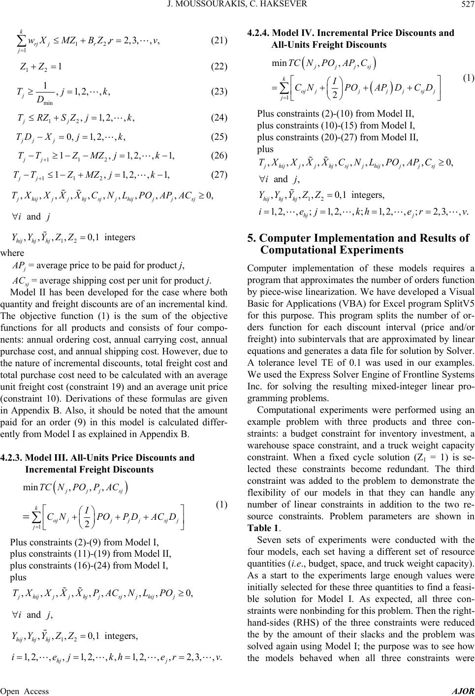 J. MOUSSOURAKIS, C. HAKSEVER Open Access AJOR 527 12 1 ,2,3,,, k rj jr j wXMZ BZrv (21) 12 1ZZ (22) min 1,1,2,,, j Tjk D (23) 12 ,1,2,,, jj TRZSZj k (24) 0,1,2,,, jj j TD Xjk (25) 112 1,1,2,,1, jj TT ZMZjk (26) 112 1,1,2,,1, jj TT ZMZjk (27) 12 ,,,, ,,,,,,0, and ,,,,0,1 integers jhij j jhjsjjhijjjsj hijhjhj TX XXXCNLPOAPAC ij YYYZZ where j P= average price to be paid for product j, j C= average shipping cost per unit for product j. Model II has been developed for the case where both quantity and freight discounts are of an incremental kind. The objective function (1) is the sum of the objective functions for all products and consists of four compo- nents: annual ordering cost, annual carrying cost, annual purchase cost, and annual shipping cost. However, due to the nature of incremental discounts, total freight cost and total purchase cost need to be calculated with an average unit freight cost (constraint 19) and an average unit price (constraint 10). Derivations of these formulas are given in Appendix B. Also, it should be noted that the amount paid for an order (9) in this model is calculated differ- ently from Model I as explained in Appendix B. 4.2.3. Model III. All-Units Price Discounts and Incremental Freight Discounts 1 min,, , 2 jjjsj k ojjjj jsj j j TC NPOPAC I CNPO PDACD (1) Plus constraints (2)-(9) from Model I, plus constraints (11)-(19) from Model II, plus constraints (16)-(24) from Model I, plus 12 ,,,,,,,,,0, and , ,,,,0,1 integers, 1, 2,,,1, 2,,,1, 2,,,2,3,,. jhijj jhjjsjjhijj hijhjhj hj j TXXXXPACNL PO ij YYYZZ iej kherv 4.2.4. Model IV. Incremental Price Discounts and All-Units Freight Discounts 1 min,, , 2 jjjsj k ojjjjjsj j j TCNPOAP C I CNPOAP DCD (1) Plus constraints (2)-(10) from Model II, plus constraints (10)-(15) from Model I, plus constraints (20)-(27) from Model II, plus 12 ,,,,,,,, ,,0, and , ,,,,0,1 integers, 1,2, ,;1,2, ,;1,2, ,;2,3, ,. jhijjjhjsjjhijjj sj hijhjhj hj j TX XXXCNLPOAPC ij YYYZZ iejkherv 5. Computer Implementation and Results of Computational Experiments Computer implementation of these models requires a program that approximates the number of orders function by piece-wise linearization. We have developed a Visual Basic for Applications (VBA) for Excel program SplitV5 for this purpose. This program splits the number of or- ders function for each discount interval (price and/or freight) into subintervals that are approximated by linear equations and generates a data file for solution by Solver. A tolerance level TE of 0.1 was used in our examples. We used the Express Solver Engine of Frontline Systems Inc. for solving the resulting mixed-integer linear pro- gramming problems. Computational experiments were performed using an example problem with three products and three con- straints: a budget constraint for inventory investment, a warehouse space constraint, and a truck weight capacity constraint. When a fixed cycle solution (Z1 = 1) is se- lected these constraints become redundant. The third constraint was added to the problem to demonstrate the flexibility of our models in that they can handle any number of linear constraints in addition to the two re- source constraints. Problem parameters are shown in Table 1. Seven sets of experiments were conducted with the four models, each set having a different set of resource quantities (i.e., budget, space, and truck weight capacity). As a start to the experiments large enough values were initially selected for these three quantities to find a feasi- ble solution for Model I. As expected, all three con- straints were nonbinding for this problem. Then the right- hand-sides (RHS) of the three constraints were reduced the by the amount of their slacks and the problem was solved again using Model I; the purpose was to see how the models behaved when all three constraints were  J. MOUSSOURAKIS, C. HAKSEVER Open Access AJOR 528 binding. This guaranteed binding constraints for Model I. The solution to this first problem with a budget amount of $110,484 is shown in the first row of Table 2. Then the same problem was solved using each of the remain- ing models. Model II produced a fixed (common) cycle solution, while the other three had independent cycle solutions. All three constraints were also binding for Model III. The same approach of manipulating the right- hand-sides in some, but not all, problems were used to create optimal solutions in which some constraints were binding. Then an additional six problems were set up and solved; the results are shown in Table 2. In solving the second problem, all tau’s (calculated outside the model) were determined to be equal, imply- ing full usage of available resources if a fixed cycle solu- tion were to be chosen as optimum, as indicated in Table 2. Furthermore, since cycle times, T’s, are the same for all models selecting a fixed cycle solution, as in the sec- ond problem, their economic order quantities are the same and can be verified by constraints (18-21) in Mo- del I, which are common to all models. Page and Paul’s [19] simulations with a single re- source constraint suggested that as the constraint gets tighter, the fixed cycle solution gives a lower total cost solution. As can be seen from Table 2, this prediction did not hold for the test problems. Independent cycle so- lutions were observed even for problems with relatively low levels of resources (Problems 6 and 7). Fixed cycle solutions, on the other hand, resulted even when resource levels were relatively high; overall, 16 of 24 problems had fixed cycle solutions. Additional experiments in- dicated that our problems had no feasible solution Table 1. Parameters of the example problem. PRODUCT 1 2 3 ANNUAL DEMAND 1600 1800 2200 COST PER ORDER (Coj) 40 90 110 HOLDING COST PERCENT (I) 0.20 0.20 0.20 SPACE OCCUPIED (w2j) 4 3 2 WEIGHT (w3j) 20 15 10 QUANTITY INTERVALS FOR PRICE DISCOUNTS (nhj, mhj) 100 - 200 50 - 150 200 - 400 201 - 500 151 - 400 401 - 800 501 - 900 401 - 1100 801 - 1400 901 - 1600 1101 - 1800 1401 - 1700 1701 - 2200 Ph1 Ph2 Ph3 PRICES ($) 40 22 55 35 20 49 32 16 45 30 14 42 40 FREIGHT DISCOUNT INTERVALS , hj hj nm 1 - 400 1 - 350 1 - 500 401 - 900 351 - 1000 501 - 1200 901 - 1600 1001 - 1800 1201 - 2200 FREIGHT COST PER UNIT ($) Csh1 Csh2 Csh3 2.00 5.00 3.50 1.90 4.50 3.00 1.70 4.20 2.50  J. MOUSSOURAKIS, C. HAKSEVER Open Access AJOR 529 Table 2. Results of computational experiments with four models (Z1 = 1 common cycle; Z2 = 1 independent cycle). TYPE OF CYCLE BUDGET ($) SPACE (CU.FT.) TRUCK CAPACITY (LBS.) X1X2X3 OBJECTIVE FUNCTION ($) UNUSED BUDGET ($) UNUSED SPACE (CU. FT.) UNUSED TRUCK CAP. (LBS.) MODEL I Z2 = 1 110,48410,309 44,937 90111011701188,389 0 0 0 MODEL II Z1 = 1 112212631543224,333 0 2690 12,758 MODEL III Z2 = 1 90111011701190,789 0 0 0 MODEL IV Z 2 = 1 11914561701227,759 0 2063 8179 MODEL I Z 1 = 1 90,4846240 26,354 91910341264202,103 0 0 0 MODEL II Z 1 = 1 91910341264227,506 0 0 0 MODEL III Z 1 = 1 91910341264204,861 0 0 0 MODEL IV Z 1 = 1 91910341264224,084 0 0 0 MODEL I Z 1 = 1 70,0004736 20,000 698785959205,103 1332 0 0 MODEL II Z 1 = 1 698785959232,905 1332 0 0 MODEL III Z 2 = 1 201401801209,350 20,504 1,127 3363 MODEL IV Z 1 = 1 698785959229,394 1332 0 0 MODEL I Z 2 = 1 50,0003500 14,563 20154801221,471 5742 933 1400 MODEL II Z 1 = 1 508571698238,189 0 52 0 MODEL III Z 1 = 1 508571698214,107 0 52 0 MODEL IV Z 1 = 1 508571698234,713 0 52 0 MODEL I Z 1 = 1 40,0002000 8447 295331405224,691 10,999 0 0 MODEL II Z 2 = 1 10056532249,732 6290 367 0 MODEL III Z 1 = 1 295331405224,722 10,999 0 0 MODEL IV Z 2 = 1 10054534247,647 6242 371 0 MODEL I Z 2 = 1 30,0003257 12,088 201166401224,602 0 1153 2603 MODEL II Z 2 = 1 100819200243,668 0 0 0 MODEL III Z 1 = 1 305343419224,809 0 1188 3350 MODEL IV Z 2 = 1 100819200242,068 0 0 0 MODEL I Z 1 = 1 20,0001500 5825 203229279237,500 0 121 0 MODEL II Z 2 = 1 130114200249,506 1290 238 334 MODEL III Z 1 = 1 203229279237,526 0 121 0 MODEL IV Z 2 = 1 11961238250,611 810 364 573 when any resource amounts are below $14,319, 988 cu. ft., and 4171 lbs. for budget, space, and truck weight constraints, respectively. A feasible solution did not exist even if only one of the resources was below its limit. However, when any resource amount was set to its limit- ing value and others at well above their limiting values, a fixed cycle solution was found with all four models. Consequently, these results may provide some support to Page and Paul’s [19] conclusion when resources are “se- verely” restricted. As resource amounts available to the supply chain manager increase, we expected our models to have lower total inventory cost solutions. This is expected, because greater resource amounts enable the model to take ad- vantage of lower unit costs and/or lower unit shipping costs by ordering larger quantities. As can be seen from  J. MOUSSOURAKIS, C. HAKSEVER Open Access AJOR 530 Table 2, this prediction turned out to be true for five of the problems, but not for Problems 2 and 6. However, Problem 6 did not conform to the pattern of decreasing resources: truck capacity increased from Problem 5 to Problem 6. Due to the advantageous nature of all-units discount schedules for buyers compared to incremental discount schedules, we expected Model I always to produce lower total cost solutions. This was true for six of the seven test problems except the fourth problem (Budget = $50,000). Similarly, we expected Model II (both incremental dis- counts) to give the highest total cost optimal solution among the four models. This prediction turned out to be true only for five problems, but not for Problems 1 and 7. 6. Summary and Conclusions The four models presented in this paper can help supply chain managers to find approximate optimal answers to the important question of “how many” to order when they make the decision for multiple products subject to multiple constraints and when quantity and freight dis- counts are available from suppliers and shippers. The four models cover all possible combinations of all-units and incremental discounts schedules for quantity and freight. We believe these models are viable tools for ma- nagers with a basic understanding of linear programming. Also, to the best of our knowledge there is no other pub- lished model that can solve the types of problems which these models can solve. The computational experiments we performed in gen- eral gave the expected results with some exceptions. Spe- cifically, whether they are for price or freight, all-units discounts schedules, in general, lead to a lower total in- ventory cost for buyers. Secondly, high resource amounts (i.e., budget, warehouse space, and truck weight capacity) at a supply chain manager’s disposal, in general, seem to lead to a lower total inventory cost. Finally, extremely low resource levels seem to lead to common cycle solu- tions for all combinations of all-units and incremental discounts. REFERENCES [1] R. Wilson, “24th Annual State of Logistics Report,” Council of Supply Chain Management Professionals, 2013. http://cscmp.org/publication-store/periodicals [2] C. Haksever and J. Moussourakis, “Determining Order Quantities in Multi-Product Inventory Systems Subject to Multiple Constraints and Incremental Discounts,” Euro- pean Journal of Operational Research, Vol. 184, No. 3, 2008, pp. 930-945. http://dx.doi.org/10.1016/j.ejor.2006.12.019 [3] W. C. Benton and S. Park, “A classification of Literature on Determining the Lot Size Under Quantity Discounts,” European Journal of Operational Research, Vol. 92, No. 2, 1996, pp. 219-238. http://dx.doi.org/10.1016/0377-2217(95)00315-0 [4] C. Munson and M. J. Rosenblatt, “Theories and Realities of Quantity Discounts: An Exploratory Study,” Produc- tion and Operations Management, Vol. 7, No. 4, 1998, pp. 352-369. http://dx.doi.org/10.1111/j.1937-5956.1998.tb00129.x [5] R. J. Tersine and S. Barman, “Lot Size Optimization with Quantity and Freight Rate Discounts,” Logistics and Transportation Review, Vol. 27, No. 4, 1991, pp. 319- 332. [6] R. J. Tersine and S. Barman, “Economic Inventory/ Transport Lot Sizing with Quantity and Freight Rate Discounts,” Decision Sciences, Vol. 22, No. 5, 1991, pp. 1171-1191. http://dx.doi.org/10.1111/j.1540-5915.1991.tb01914.x [7] F. J. Arcelus and J. E. Rowcroft, “Inventory Policies with Freight Discounts and Disposals,” International Journal of Operations & Production Management, Vol. 11, No. 4, 1991, pp. 89-91. http://dx.doi.org/10.1108/01443579110143197 [8] M. Diaby and A. Martel, “Dynamic Lot Sizing for Multi- echelon Distribution Systems with Purchasing and Trans- portation Price Discounts,” Operations Research, Vol. 41, No. 1, 1993, pp. 48-59. http://dx.doi.org/10.1287/opre.41.1.48 [9] R. J. Tersine, S. Barman and R. A. Toelle, “Composite Lot Sizing with Quantity and Freight Discounts,” Com- puters and Industrial Engineering, Vol. 28, No. 1, 1995, pp. 107-122. http://dx.doi.org/10.1016/0360-8352(94)00031-H [10] T. H. Burwell, D. S. Dave, K. E. Fitzpatrick and M. R. Roy, “Economic Lot Size Model for Price-Dependent Demand under Quantity and Freight Discounts,” Interna- tional Journal of Production Economics, Vol. 48, No. 2, 1997, pp. 141-155. http://dx.doi.org/10.1016/S0925-5273(96)00085-0 [11] M. A. Darwish, “Joint Determination of Order Quantity and Reorder Point of Continuous Review Model under Quantity and Freight Rate Discounts,” Computers & Op- erations Research, Vol. 35, No. 12, 2008, pp. 3902-3917. http://dx.doi.org/10.1016/j.cor.2007.05.001 [12] A. Mendoza and J. A. Ventura, “Incorporating Quantity Discounts to the EOQ Model with Transportation Costs,” International Journal of Production Economics, Vol. 113, No. 2, 2008, pp. 754-765. [13] A. Toptal, “Replenishment Decisions under an All-Units Discount Schedule and Stepwise Freight Costs,” Euro- pean Journal of Operational Research, Vol. 198, No. 2, 2009, pp. 504-510. http://dx.doi.org/10.1016/j.ejor.2008.09.037 [14] W. C. Benton, “Quantity Discount Decisions under Con- ditions of Multiple Items, Multiple Suppliers and Re- source Limitations,” International Journal of Production Research, Vol. 29, No. 10, 1991, pp. 1953-1961. http://dx.doi.org/10.1080/00207549108948060 [15] P. A. Rubin and W. C. Benton, “Jointly Constrained Or-  J. MOUSSOURAKIS, C. HAKSEVER Open Access AJOR 531 der Quantities with All-Units Discounts,” Naval Research Logistics, Vol. 40, No. 2, 1993, pp. 255-278. http://dx.doi.org/10.1002/1520-6750(199303)40:2<255:: AID-NAV3220400209>3.0.CO;2-G [16] P. A. Rubin and W. C. Benton, “Evaluating Jointly Con- strained Order Quantity Complexities for Incremental Discounts,” European Journal of Operational Research, Vol. 149, No. 3, 2003, pp. 557-570. http://dx.doi.org/10.1016/S0377-2217(02)00457-5 [17] F. Guder, J. Zydiak and S. Chaudhry, “Capacitated Mul- tiple Item Ordering with Incremental Quantity Dis- counts,” Journal of the Operational Research Society, Vol. 45, No. 10, 1994, pp. 1197-1205. [18] M. J. Rosenblatt, “Multi-Item Inventory System with Budge- tary Constraint: A Comparison between the Lagrangian and the Fixed Cycle Approach,” International Journal of Production Research, Vol. 19, No. 4, 1981, pp. 331-339. http://dx.doi.org/10.1080/00207548108956661 [19] E. Page and R. J. Paul, “Multi-Product Inventory Situa- tions with One Restriction,” Operational Research Quar- terly, Vol. 27, No. 4, 1976, pp. 815-834. [20] F. Güder and J. Zydiak, “Fixed Cycle Ordering Policies for Capacitated Multiple Item Inventory Systems with Quantity Discounts,” Computers and Industrial Engi- neering, Vol. 38, No. 3, 2000, pp. 67-77. http://dx.doi.org/10.1016/S0360-8352(00)00029-2 [21] J. Moussourakis and C. Haksever, “A Linear Approxima- tion Approach to Multi-Product Multi-Constraint Inven- tory Management Problems,” Tamsui Oxford Journal of Management Sciences, Vol. 20, No. 1, 2004, pp. 35-55.  J. MOUSSOURAKIS, C. HAKSEVER Open Access AJOR 532 Appendix A Linear Approximation of the Number of Orders Function The number of orders function is strictly convex and can be approximated with a series of linear functions. In the presence of quantity discounts this function should be viewed as consisting of segments corresponding to dis- count intervals (Figure 1). Consider such a segment of the function approximated by a linear function (Figure 2). The error of estimation, Ehij, for subinterval i of quan- tity discount h for product j is given by hij hijj hijhij hijjhij ELN abX DX (A.1) The maximum error can be reduced to any finite num- ber by increasing the number of line segments. Once the maximum error a decision maker is willing to tolerate (TE) is determined, the next task is to split each quantity discount interval into as many sub-intervals of order quantities (X) as necessary so that no line segment over- estimates N by more than TE. An efficient way is to split the intervals at the point where the error Ehij is at maxi- mum, thereby reducing overestimation by the greatest amount. Suppose we start with the first discount interval as in- terval 1, which is approximated by the line segment 1111 p ijijij ij LabX , where the superscript p represents the iteration number and is set equal to 0 at the beginning of the process (Figure 2). Since the process can be ap- plied to only one discount interval of one product at a time, the subscripts h and j will be dropped in the discus- sion. Also, some values will be identified by the iteration at which they are calculated. For example, (2 ) 1 repre- sents the slope of the line that approximates the curve in subinterval 1 at the second iteration. We assume that the range of N values a decision maker wants to consider is determined by the range of discount intervals; if the up- per limit of the last (i.e., lowest price) interval is open, as is usually the case, it is set equal to SD. Therefore, the range of N values for each product will be from (1/S) to D. However, since we will be linearizing the function separately for each quantity discount interval, the range of N values will be determined by the discount schedule. For example, ordinates of the first discount interval for product j can be determined as 0 11L NDn , and 0 11R NDm for the left and right end points, respec- tively, where 0 11 j nq, and 0 12 j mq, quantities that define the first discount interval. From Equation (A.1), and by ordinary differentiation, the error for any subinterval i, Ei, is maximum at io i Db with the corresponding io i NDb; where the subscript o refers to the point at which the er- ror of estimation is maximum (Emax). For any subinterval i, let iL i NDn and iR i NDm represent the ordinates of the left and right end points, respectively. Then, given the coordinates of the end points (ni, NiL) and (mi, NiR) of any subinterval i, the equation of a line segment iiii LabX (A.2) passing through these end points can be constructed: iL iR iii NN bnm (A.3) iL iR iii ii NN aXL nm . (A.4) The value of ai can be calculated by substituting the coordinates of one of the end points of the subinterval in (A.5) as explained shortly. The maximum error, maxi E, for any subinterval i, can be computed as max 2 ii i EaDb . (A.5) by substitution of io i Db and io io NDX in Equation (A1). If the maximum error is above the tolerable error (TE), the subinterval will be split into two at Xio. Let’s assume that EiMax TE for the first discount interval; hence, we split this interval into two subintervals at 0 11 o Db. The coordinates of the end points of the two newly con- structed subintervals are (Figure 2): Subinterval 1: 1 11111 11111 1 00 11 , and , or , and , LR nNmN nDn Db Db (A.6) Subinterval 2: 11 11 2222 1 00 1 11 22 , and , or , and , LR nN mN DbDbm Dm (A.7) where 11 0 12 1 o mnX , and 1100 1211 RLo NNN Db . Also, note that the left end of the first subinterval and the right end of the last subinterval of a discount interval will always remain the same regardless of the number of subintervals created. These are the end points that de- fined the first discount interval at iteration 0. In other  J. MOUSSOURAKIS, C. HAKSEVER Open Access AJOR 533 Figure 2. Splitting the first discount interval. words, set 10 111 j nnq and 10 212 j mmq . The next step would be to construct the equations of the lines approximating the newly created subintervals. The slope and the y-intercept can be calculated according to equa- tions (A.3) and (A.4) and by substitution from (A.6) 10 11 111 11 111 10 11 11 LR Dn Db NN bnmnDb (A.8) 10 11 11 11 1 11111 10 11 Dn Db a bXLXL nDb . (A.9) To calculate the value of 1 1 a we need to evaluate equation 1 1 L at either end point of the subinterval it approximates. For example, if we evaluate 1 1 L at the right end of the first interval, we know from (A.7) that 10 11 LDb and 0 11 o Db. Substituting these values in (A.9) 1 1 a will be determined 10 100 11 111 10 11 Dn Db aDbDb nDb . (A.10) Similarly, the slope and y-intercept for the line seg- ment approximating the second subinterval can be cal- culated, for example, using the coordinates of its left end, as 1 0 11 112 22 211 01 22 12 LR DbD m NN bnm Db m (A.11) 1 0 100 12 211 01 12 DbD m aDbDb Db m . (A.12) Next, we calculate the maximum error and check if it is below TE. For example, the maximum error for the two subintervals created at the end of Step 1 would be:  J. MOUSSOURAKIS, C. HAKSEVER Open Access AJOR 534 11 1max11 2Ea Db and 11 2max22 2Ea Db . This process of splitting discount intervals into subin- tervals can be repeated until the maximum error in every interval or subinterval is below TE. For a more detailed discussion of this algorithm, see Moussourakis and Hak- sever [21]. Appendix B Computation of Average Price (AP) and Total Purchase Cost of an Order (PO) Holding cost is assumed to be a percentage (I) of the amount paid for an order and can be calculated as I(AP)(X/2) for each product. However, a straightforward computation of the average cost would introduce nonlin- earities into the objective function. In order to avoid this situation we compute the average price as follows: 112 21 33 21 1 hjjjjjj j jjjhjj hj APPUPUU X PUUPX U 11222 133 32 1 1 hjjjj jjjjj j jjhjj hj hj P PUPUPUPU X PUPXPU 1122 23 11 1 hjj jjjjj j hjhj j hj hj PUPPUPP X UPPPX 1 1 1 1 1; ; 1,2,,;2,3,, h hjqj qjhj qj q j hj j hj APUPPP X UXUj khe , where 11jj PP, hj AP average price per unit paid if the hth discount interval has been adopted, hj U = upper end point of discount interval ,1,2,, j hh e, hj P price to be paid for the units that are in discount interval ,1,2,,. j hh e Total purchase cost for product j can be computed as 1 1 1 1h jqjqj jj qj hj q j PDUPPPX D X , where h* = adopted discount interval. Let 1 1 1 , 1,2,,;2,3,,, h hjqj qjj qj q UPP jkhe 101,2,,,, j jk hj = constant inputs, calculated outside the model. Then, substituting NjXj for Dj, hj jj jj hj j jjjj hj hjhj hj g APDPN X X NPNX gNPD hence, 1 jj hj hj j PgNP D . Since Nj is defined as: 11 jhj ee hij hi NL , substituting this expression into the formula for APj, and facilitating the picking of the price for the adopted discount interval through Yhj lead to constraints 11 1 1,1,2,, . jhj j ee e jhjhijhj hj hi h j PgLPYjk D Relying on the above stated relationships, POj, total dollar amount to be paid for one order of product j, can be determined: 1 1 1 1 jjj h qj qjjj qj hj jq POAP X UPPXPX X 1 1 1 h qj qjjj qj hjhjhj q POUPPP XgPX . And finally constraints POj can be obtained as: 111 ,1,2,,. jjhj hj eee jhjhjhij hhi POgYPXjk Similar to the computation of the total purchase cost, the total shipping cost for product j can be calculated as 1 1 1 1, h jj qjsqjjj sq jsh j q j CDUCCC XD X where adopted discount interval,h and 1 1 1 ,1,2,,; 2,3,, , h qj sqjsq j q j UC Cjk hj he  J. MOUSSOURAKIS, C. HAKSEVER Open Access AJOR 535 10,1, 2,,, j jk hj = constant inputs, calculated outside the model, and following a similar procedure to the one used for APj, , hj sjjjj sh j j jj jj hj shjhjshj g ACDCN X X NCNXgNCD where 11 , jhj ee hij hi NL average shipping cost can be calculated: ** * 11 1 1 11, 2,,. jhjj sj j hj shj j eee hj hijhj sh j hi h j ACgNC D LCYj k D ,
|