Paper Menu >>
Journal Menu >>
 iBusiness, 2013, 5, 69-73 http://dx.doi.org/10.4236/ib.2013.53B015 Published Online September 2013 (http://www.scirp.org/journal/ib) 69 Theoretical Analysis of Financial Portfolio Model Xingang Wang Graduate School of Northeast Forestry University. Email: 920028102@qq.com Received June, 2013 ABSTRACT This article introduces portfolio selection model proposed by Markowitz in 1952, as well as research of model pro- moted continually by subsequent researchers, and then introduces a more classic pricing model CAPM in stock market, and discusses difficulties in the study of modern portfolio theory, and forecasts problems of benefits and risks. Keywords: Portfolio; CAPM; Benefits and Risks 1. Portfolio Selection Model Portfolio (portfolio) refers to that different investor assets are grouped together by a certain percentage as an in- vestment, and stocks, bonds, discharge capacity, collecti- bles, and other objects can be part of portfolio as an in- vestment. Portfolio Theory discusses the interrelation between each asset and other assets of risk and return, and how investors choose their optimal portfolio reason- able and other issues. 1) Standard portfolio model Before H. Markowitz founded the modern theory of portfolio, Western financial asset investment theory has experienced more than a century. After World War II, Western nations suffered rapid economic recovery and investment activities of financial assets also would be booming. In the context of this reality, Markowitz founded portfolio selection theory. Markowitz used ma- trix algebra, vector spaces, probability and statistics and other mathematical methods, to do qualitative and quan- titative analysis of portfolio selection theory in portfolio investment. Portfolio is an effective way to diversify investment risks. In 1952 Markowitz published a classic paper Port- folio Selection, and laid the basis for Portfolio theory, and thus won the Nobel Prize in economics. Purpose of portfolio selection model proposed by Markowitz is to diversify investment risks essentially under the premise of maximizing without loss of yield. He pointed out that the risk of the portfolio not only depends on features of individual securities, [1]but also on correlation between securities in the securities portfolio. Generally speaking, the lower the correlation between securities is; the lower the portfolio's risk is. In Markowitz’s theory, the Evaluation indexes of Risk Securitization are thus two, named investment average yield µ and yield variance σ², μ are the Evaluation in- dexes of the securities profitable size, and σ ² are securi- ties risk indicators. Investors can use the following mod- els to determine the optimal portfolio. Optimal portfolio can be determined by the following model Model A Min aª=x²Ώx x²-µ=µ° x²-e=1 Where X is the variance of securities investment rate of return, n securities investment ratio vector is X, the covariance matrix X is n kind of stock returns, X is n kind of bond yields mean vector, X elements for 1 n-dimensional vector, for the portfolio expected rate of return. Model A fails to consider the negative investment proportional coefficient, due to the negative investment ratio means selling the relevant securities, and short sell- ing in some occasions, especially in difficult to realize our country, so it is necessary to consider the case of no short sale. Model B Min a²=X²ΏX X¹-µ=µ X¹-en=1 X>0 Model A and model B are allowing short-selling or not under the conditions of the Makovecz mean ---- variance model. Their meaning is: In the given securities invest- ment is expected to yield under X conditions, the securi- ties portfolio investment risk. Based on the X positive definite, [2]and its corresponding organization invest- ment risk optimal model of A solution. Copyright © 2013 SciRes. IB  Theoretical Analysis of Financial Portfolio Model 70 At present there is no analytical model of B, but the domestic and foreign experts have proposed some algo- rithm, tree algorithm to improve the solution model of B optimal solutions are given. The optimal model A and model B solutions usually can be used as an effective portfolio. But because the expected variance models es- pecially the computational complexity of model B, so far in solving large-scale investment securities organizations are still restricted. Some scholars in order to solve this problem using a similar linear programming technique or index model to reduce the parameters to be estimated. Also some scholars use the income difference, deviation as a measure of risk, in order to simplify the calculation. Below is a brief introduction of several other models 1) Max Standard Analysis Due to the law and policies, there are some propor- tions or limitation in total amount for securities groups in single or all securities investments. If such limitation differs to every security, then the following constraint sets are listed: n ΣXi =1 t=1 Xt ≧ 0,i =1,...,n Xt ≦ Ui, i=1,...,n All these constraint sets above are the same as that of standard portfolio selection mode except the max in- vestment number Ui (it is assumed as a constant) of each securities. The max standard analysis is an exception of portfolio selection mode. 2) Tobin-Sharp-Lintner Model Tobin-Sharp-Lintner Mode allows to considering the other flow direction of capitals. However, there is a premise that is the flowing out amount of money can not overpass its own amount but the flowing in money has no limitation. Therefore, portfolio selection is restricted by the following items: n ΣXi =1+Xn+1 i=1 Xi ≧ 0,i=11,...n Xn+1 ≧ -1 or it can be written as n ΣXi -Xn+1=1 i-1 Here it should be noticed that the limitation of Xn +1 is not 0 but -1. In the analysis of Tobin (1958), Sharp (1964) and Lintner (1965), the variable Xn+1 represents bor- rowing if it is a positive number and loan if it’s a nega- tive number. As for the variance Vn+1=σn+1, if n+1 is 0, then i=1, ... , n, σn+1 equals 0 as well. Usually, the rate that a investor get form the loan and borrowing refers to the risk-free rate. It can be expressed as γ0. Since Xn+1 means the borrowing money, μn+1 = -γ0. 3) Model for Bear Position That Need Attachment Mortgage If the variable has no non-negative limitation, i.e, only under the condition of ΣXi =1, the following feasible solutions may appear: X1 = -1000 X2 = +1001 Xi = 0 i = 3, ..., n The answers above mean the 1000 unit bear of securi- ties 1 and the 1001 unit bull of securities 2. In fact, it is impracticable for individual, investment institution or brokerage. According to the law, mortgage is a must. Thus, the constrained items can be showed in the fol- lowing ways: K+G ΣXi L ≦ A i=1 K+G K+G aΣXi S ≦ A + ΣXi i=1 i=1 XiL ≧0, i =1, ... , K+G XiS ≦0, i =1, ... , K+G A here means assets; XiL means the bull position of securities i; XiS means bear position of securities i. The money that total number multiplies a which means the require of mortgage should not surpass the money that right capital surpluses the bear value which can’t be used as mortgage, i.e the Securities K. 2. Capital Assets Pricing Model Capital Assets Pricing Model, short for CAPM, is found and raised single and respectively by William F. Sharpe, an American economist who won the Nobel Economics Prize in 1990, John Linter and Jack Treynor. This model is at the core of capital market theories and it’s a signifi- cant achievement of modern financial theories and secu- rities theories. This model attaches great importance to guiding the securities investment. 1) Assumptions of CAPM CAPM is developed from the portfolio selection and the assumptions about which are more rigorous than capital group theories. The basic assumptions are listed as follows: a) All investors are risk aversion. They weight the gains or risks or assets with the expected value or vari- ance or standard deviation of the asset returns. b) Investors determine the investment based on the single gains and risks and the investment horizon are the same. c) There’s no obstacle in securities market, which means the transacting fees are zero. The transacting amount of assets is divisible. Investors can buy any asset Copyright © 2013 SciRes. IB 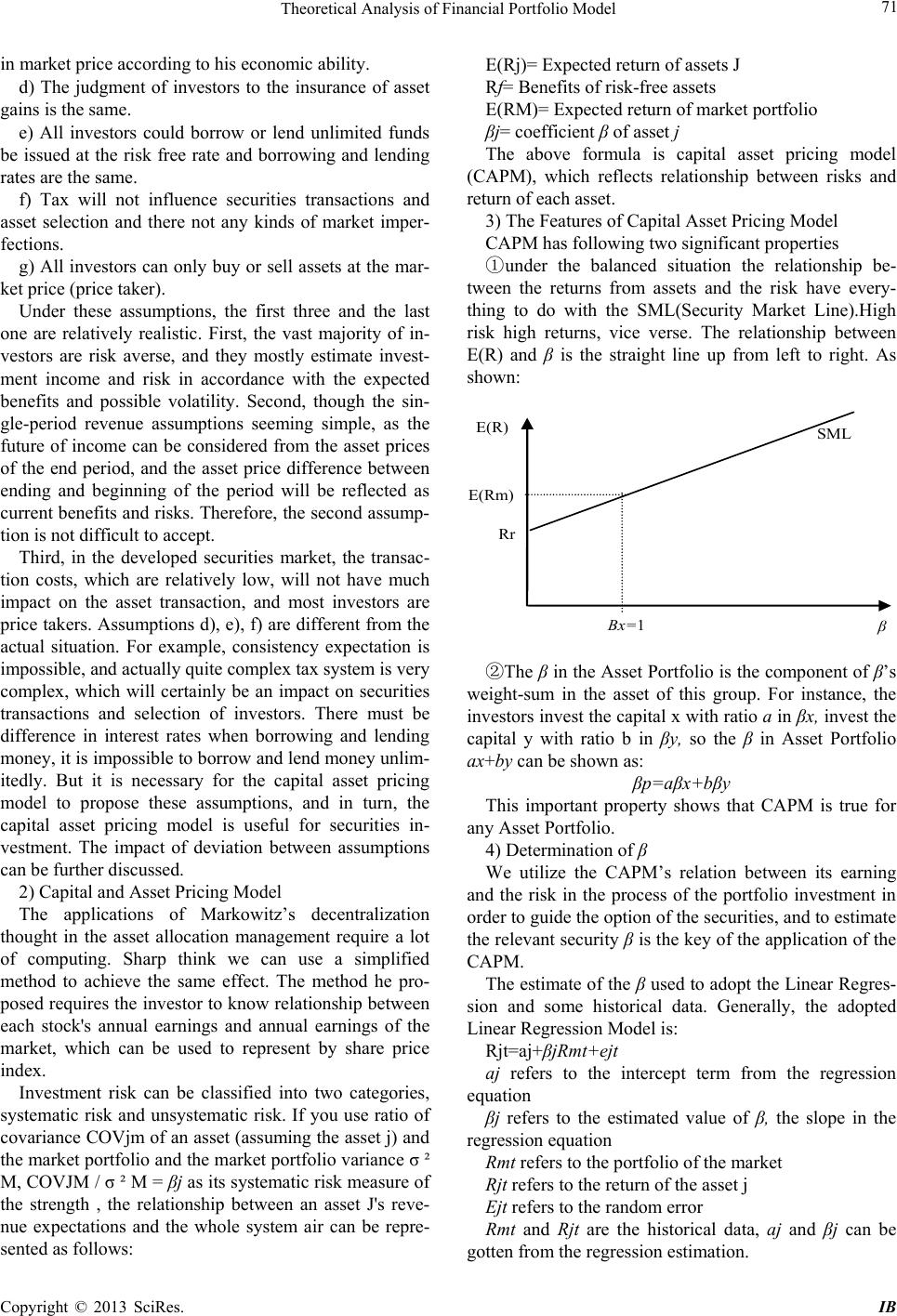 Theoretical Analysis of Financial Portfolio Model 71 in market price according to his economic ability. d) The judgment of investors to the insurance of asset gains is the same. e) All investors could borrow or lend unlimited funds be issued at the risk free rate and borrowing and lending rates are the same. f) Tax will not influence securities transactions and asset selection and there not any kinds of market imper- fections. g) All investors can only buy or sell assets at the mar- ket price (price taker). Under these assumptions, the first three and the last one are relatively realistic. First, the vast majority of in- vestors are risk averse, and they mostly estimate invest- ment income and risk in accordance with the expected benefits and possible volatility. Second, though the sin- gle-period revenue assumptions seeming simple, as the future of income can be considered from the asset prices of the end period, and the asset price difference between ending and beginning of the period will be reflected as current benefits and risks. Therefore, the second assump- tion is not difficult to accept. Third, in the developed securities market, the transac- tion costs, which are relatively low, will not have much impact on the asset transaction, and most investors are price takers. Assumptions d), e), f) are different from the actual situation. For example, consistency expectation is impossible, and actually quite complex tax system is very complex, which will certainly be an impact on securities transactions and selection of investors. There must be difference in interest rates when borrowing and lending money, it is impossible to borrow and lend money unlim- itedly. But it is necessary for the capital asset pricing model to propose these assumptions, and in turn, the capital asset pricing model is useful for securities in- vestment. The impact of deviation between assumptions can be further discussed. 2) Capital and Asset Pricing Model The applications of Markowitz’s decentralization thought in the asset allocation management require a lot of computing. Sharp think we can use a simplified method to achieve the same effect. The method he pro- posed requires the investor to know relationship between each stock's annual earnings and annual earnings of the market, which can be used to represent by share price index. Investment risk can be classified into two categories, systematic risk and unsystematic risk. If you use ratio of covariance COVjm of an asset (assuming the asset j) and the market portfolio and the market portfolio variance σ ² M, COVJM / σ ² M = βj as its systematic risk measure of the strength , the relationship between an asset J's reve- nue expectations and the whole system air can be repre- sented as follows: E(Rj)= Expected return of assets J Rf= Benefits of risk-free assets E(RM)= Expected return of market portfolio βj= coefficient β of asset j The above formula is capital asset pricing model (CAPM), which reflects relationship between risks and return of each asset. 3) The Features of Capital Asset Pricing Model CAPM has following two significant properties ①under the balanced situation the relationship be- tween the returns from assets and the risk have every- thing to do with the SML(Security Market Line).High risk high returns, vice verse. The relationship between E(R) and β is the straight line up from left to right. As shown: E(R) SM L E(Rm) R r Β x =1 β ②The β in the Asset Portfolio is the component of β’s weight-sum in the asset of this group. For instance, the investors invest the capital x with ratio a in βx, invest the capital y with ratio b in βy, so the β in Asset Portfolio ax+by can be shown as: βp=aβx+bβy This important property shows that CAPM is true for any Asset Portfolio. 4) Determination of β We utilize the CAPM’s relation between its earning and the risk in the process of the portfolio investment in order to guide the option of the securities, and to estimate the relevant security β is the key of the application of the CAPM. The estimate of the β used to adopt the Linear Regres- sion and some historical data. Generally, the adopted Linear Regression Model is: Rjt=aj+βjRmt+ejt aj refers to the intercept term from the regression equation βj refers to the estimated value of β, the slope in the regression equation Rmt refers to the portfolio of the market Rjt refers to the return of the asset j Ejt refers to the random error Rmt and Rjt are the historical data, aj and βj can be gotten from the regression estimation. Copyright © 2013 SciRes. IB  Theoretical Analysis of Financial Portfolio Model 72 3. The Issues about the Gain and Forecast in Security Portfolio Theory Among the various kinds of theories about the option of Security Portfolio the further gain and variance are the basis of the decision. And it’s a difficult point of the pre- sent study that how to forecast the security portfolio. As the security portfolio is a random variable so it’s will not just a simple repetition. The historical data is insufficient for some investment projects or assets, especially emerging industries which because of the changes of the economic development, policies and etc. So the forecast by the historical data like ‘driving by the rear-vision mirror’, [3] so the effect is unsatisfactory phenomenon. There is no investor can forecast the further gain of the securities precisely, from this point, there are two Bayes- ian methods which suitable to the analysis of the securi- ties of the financial market: fundamental analysis and technical analysis 1) Fundamental analysis Fundamental analysis, is the analysis and study of the securities, especially the stock, and put priority in the intrinsic value of the securities. By analysis the macro- investmental environment, especially the basic case of economic environment, the publisher’s industry, to seek the value of the securities and decide whether it’s worthy to be invested. The change of the securities’ price can be caused by several reasons. In political, the war the political turmoil the leadership change and so on, will affect the investor’s confidence more or less and then affect the stock market; in economic aspect ,the economic growth the inflation the change of the interest rate the exchange rate all of them will have an effect on the stock market. National policies such as control the money supply, adjustment of tax, rate of tax, to support, lean or restrict to an industry and etc, all will affect the stock price. So keep a close eye on the change of the macro-politics and economy is very important for the analysis and study. Industry analysis refers to analyzing the issuer and the listing Corporation out of what kind of industry and the company is in the status of the industry. The company position in the industry is also very important, in differ- ent position in the same industry, its ability to grow dif- ferent. The company's high status, high visibility, easy to obtain the stable and huge profits, but its growth ability may be weak. The position of the lower company, visi- bility is not high; the lack of competitiveness, but future growth capacity may be strong. Growth firms are a better choice for investors. Analysis of the company itself is the most important part of the basic analysis. [4]To include many aspects analysis company, such as the products of the company, in what the product cycle, market share, new product development ability. The key to the analysis of the com- pany’s marketing efficiency, production efficiency and management efficiency. Through the analysis of financial indicators, such as the balance sheet, income statement, marketing situation analysis of the company’s, the com- pany also analysis of stability, activity ability, profit abil- ity, growth ability through the company's other indica- tors. In short, the basic analysis method is refers to the use of statistical data, using a variety of economic indicators, the proportion, method of dynamic analysis, from the macro political, economic, to the industry analysis, until the business profit status and Prospect of micro analysis, evaluation of enterprises issued by the securities, and as far as possible to predict its future change, as investors investment basis. 2) Technical analysis Technical analysis is based on the statistical data of the future past stock market movements. [5]Technical analy- sis is purely focused on the analysis of price and the quantity of securities, without considering the company's financial position and profitability. According to the price and trading volume change, to predict the stock price up or down, to determine the behavior of invest- ment. This method considers all affect securities, espe- cially various kinds of factors of stock, will be reflected in the price level and stock trading volume. If the phe- nomenon of certain activities, the market price changes, including the cycle has appeared in the past, is very likely to appear again in the future. History will repeat itself. Technical analysis method mainly through statistical quantity price and trading of securities. This analysis method is developed to today, can be said to be rich and colorful, perfection. Such as Dow Theory, the moving average line, K line graph, chart, and bar chart. Fundamental analysis and technical analysis have strengths; they analyze the stock market from a different perspective, reflecting the change of the stock market to a certain extent. Difference between fundamental analy- sis and technical analysis: the former is mainly to look forward, pay attention to the future earnings and risk; the latter mainly look back, to the market already happening to predict future basis. In practical analysis, should be to combine the two organic. Through the analysis of the previous price data, [6]the future trend can be predicted. However, the basic analy- sis for the importance of stock prediction can not be ig- nored. Therefore, the Bayesian method is proposed in this paper, which embodies the idea: according to the latest news, including the expert experience and subjec- tive judgment, revised historical data model. Through the analysis of the previous price data, we can predict the future trend. However, the importance of basic analysis for the stock prediction can not be ignored. Copyright © 2013 SciRes. IB  Theoretical Analysis of Financial Portfolio Model Copyright © 2013 SciRes. IB 73 Therefore, the Bayesian method is proposed in this paper, which embodies the idea: according to the latest news, including the expert experience and subjective judgment, revised historical data model. REFERENCES [1] H. C. John, “The Risk and Return of Ventufe Capital,” Tournal of Fimamcics, Vol. 75, No. 1, 2005, pp. 3-52. [2] Y. Y. Lao, Financial Securities, Beijing. Economic Man- agement Publishing House, 2003. [3] G. Lee, Financial Economics, Chengdu. Sichuan Univer- sity press, 1999. [4] Y. Lu, Financial Market Investment Decision Optimiza- tion in Probability Criterion, the Heilongjiang Province Natural Science Fund Project (G0521), 2008. [5] Y. F. Meng, “Securities Investment,” Xiamen. Xiamen University press, 2006 [6] J. Y. Wang, Application of Statistics. Harbin. Heilongji- ang People's Publishing House, 1999. |