Communications and Network, 2013, 5, 103-107
http://dx.doi.org/10.4236/cn.2013.53B2020 Published Online September 2013 (http://www.scirp.org/journal/cn)
Dynamic K-Best Sphere Decoding Algorithms for
MIMO Detection
Chengzhe Piao, Yang Liu, Kaihua Jiang, Xinyu Mao
School of electronic engine e r ing and comp u t er science, Peking University, Beijing, China
Received May, 2013
ABSTRACT
Multiple Input Multiple Output (MIMO) technology is of great significance in high data rate wireless communication.
The K-Best Sphere Decoding (K- Best SD) algorithm was proposed as a powerful method for MIMO detection that can
approach near-optimal performance. However, some extra computational complexity is contained in K-Best SD. In this
paper, we propose an improved K-Best SD to reduce the complexity of conventional K-Best SD by assigning K for
each level dynamically following some rules. Simulation proves that the performance degradation of the improved
K-Best SD is very little and the complexity is significantly redu ced.
Keywords: Multiple Input Multiple Output (MIMO); Detection; K-Best Sphere Decoding (K-Best SD)
1. Introduction
Multiple-input multiple-output (MIMO) system, which
utilizes the spatial div ersity, has been extensively studied
during the past decade, because it has high spectral effi-
ciency [1]. The optimal performance of MIMO system
detection can be achieved by maximum likelihood (ML)
detection algorithm based on exhaustive search. However,
the computational co mplexity is significantly affected by
the size of modulation constellations and the antenna
numbers. It increases exponentially with them. In order
to decrease the computational complexity and apply in
hardware, an improved algorithm, called the sphere de-
tection algorithm (SD), is studied in [2,3]. The SD can
offer a performance near maximum-likelihood algorithm
with an acceptable complexity.
In the SD, detection is transformed into a depth-first
tree search problem. This leads to a disadvantage that the
computational complexity varies so obviously with dif-
ferent signals and channels that implementations of SD
will be inconvenient. Hence the K-Best algorithm based
on the breadth-first tree search strategy is put forward
[4-5]. In the K-Best algorithm, only the best K candidates
at each level of tree are reserved for further search in
next level. This eliminates the disadvantage above. The
fixed computational complexity makes implementation
easily. However, comparing with ML algorithm, the K-
best algorithm suffers performance degradation espe-
cially when K is small. It is because a larger value of K
makes it less possible that the K-Best solution is not
equal to the ML solution. The existing K-Best algorithm
cannot meet the increasing need for low computational
complexity and high data rate of MIMO system.
In view of above, we proposed a new dynamic K-Best
algorithm in this paper. In con ventional K-best algorithm,
a set consisted of K candidates, which have the smallest
Euclidean distances, is kept for search in the next level.
The difference between the smallest Euclidean distance
and second smallest Euclidean distance is related to the
possibility that the K-best solution is near to the ML so-
lution. In the proposed algorithm, the value of K can be
adjusted accord ing to the difference so that the computa-
tional complexity is significantly reduced with small,
even negligible, performance degradation.
The remainder of this paper is organized as follows. In
section 2, the fundamental model of MIMO system is
introduced. And we will review several basic decoding
algorithms. In section 3, we will introduce the main ideas
of sphere decoding (SD) algorithms. In section 4, we will
describe our dynamic K-best algorithms in detail. In sec-
tion 5, we will present our simulation results to demon-
strate its complexity decrease. In section 6, the conclu-
sion will be drawn.
2. Background Review
2.1. MIMO System Model
Consider a MIMO system with NT transmit antennas and
NR receive antennas and assume that channel of this sys-
tem is a Rayleigh fading channel. The relationship be-
tween the transmitted signal and received signal can be
described as follows:
C
opyright © 2013 SciRes. CN

C. Z. PIAO ET AL.
104
(1)
in which denotes the dimen-
sional received signal vector and
denotes the NT dimensional transmitted signal vector.
And the no ise vector is a complex
zero-mean additive Gaussian noise vector with variance
per dimension. Its powers of real parts and imaginary
parts are equal. The flat fading channel is described by a
complex matrix .
(2)
The element of channel matrix stand for the path
gain from the transmit antenna to the receive
antenna. It is supposed that channel matrix is fully
known by receiver. Meanwhile, in order to simplify the
calculation, we assume that = = .
The complex channel matrix, transmit vector, receive
vector, and noise vector can be transformed into its real
representation.
(3)
(4)
where stands for the real part and stands for
the imaginary part.
Utilizing these real representations, (1) is transformed
into (5)
2.2. ZF Decoding
The Zero-Forcing (ZF) Decoding result is given by
(6)
where is the Moore-Penrose in-
verse of the channel matrix H [6]. ZF decoding trans-
forms the joint decoding into single stream decod-
ing so as to reduce the complexity significantly. However,
the reduction comes at the expense of large noise ampli-
fication leading to a much worse performance.
2.3. ML Decoding
The ML performance is optimal. For the receiver, the
conditional probability destiny function in
the case of a Gaussian channel is given by
(7)
with [7]. Therefore, maximizing the
conditional pdf amounts is equal to minimizing
because the other terms are constant
factors. So the mathematical model of ML detection is
(8)
where is the set of all transmitted vectors .
For MIMO systems with N transmit antennas and the
modulation order of m, contains elements, and
obviously ML Decoding using exhaustive search must
search the whole set to find the optimal solution .
Hence the complexity of ML Decoding increases expo-
nentially with the product of m and N , so for large con-
stellations and large N ML Decoding is impractical.
3. Sphere Decoding
3.1. Sphere Decoding
As is mentioned above, the ML detection based on ex-
haustive search is difficult in practice. Therefore a re-
striction of searching space is necessary. The SD is ef-
fective in reducing the complexity of ML detection by
means of enumerating the lattice points within a distance
lower than a given maximum named sphere radius.
So the mathematical description of SD is
(9)
Here is a subset of the searching space of ML.
But unfortunately, th is kind of SD is not stable enough in
that it cannot redu ce much complexity if is too large,
and on the other hand, it easily discards the ML solution
at early stages of searching if is too small [8].
In order to simplify the searching, a decoding tree is
usually employed. To create such a tree, an upper train-
gular structure R of the channel matrix H obtained by
QR decomposition is required. Using QR decomposition,
the MIMO channel model can be rewritten as below:
(10)
or (11)
Since Q is a unitary matrix, it can maintain the statis-
tical characteristics of noise vector n. Thus the new sys-
tem is equivalent to the former one. In this way, the re-
newed expression of SD is
(12)

C. Z. PIAO ET AL. 105
Here j is the level number of the tree and N is the
number of antennas of the transmitter and the receiver.
The nodes of the tree store the information of the partial
solutions in order to find the op timal solution. Th e squ are
of the Euclidean distance, namely , is cal-
culated by computing partial Euclidean distance (PED)
for each level j, i.e.
(13)
Obviously (14)
3.2. Depth-First SD
The Depth-First Sphere Decoding algorithms contain
forward and backward directions of searching the tree. It
is carried out as below:
1) Set a large number as optdist (distance of the opti-
mal solution);
2) Go forward to the first leaf of the tree;
3) Calculate the lowest distance of the nodes expanded
by the same node with the leaf to update the optdist;
4) Go back to the former level and try the next node; if
the end of nodes is reached, continue this step until there
is a node available; if no such node exists, go to step 7.
5) If the PED of the node is larger than optdist, then go
to step 4; else expand the node and go to step 6;
6) If the leaf is reached, go to step 3; else go to step 5.
7) Choose the solution whose PED is optist as the op-
timal solution.
3.3. Fixed K-Best SD
Compared with exhaustive search, K-Best SD uses
Breadth-First Search (BFS). BFS only allows forward
direction and the information of nodes at current level
will be kept before the nodes are expanded. K-Best algo-
rithm keeps only K nodes at each level. Let j be the level
number. The procedure of the algorithm is:
1. Let j = N;
2. Calculate the PEDs of all nodes at level j expanded
by the former level and choose smallest
ones, where is the number of nodes at level j;
3. Expand the chosen nodes, and ;
4. If , go to step 2; else go to step 5;
5. Choose the smallest PED as the optimal solution.
4. Dynamic K-Best Algorithm
The fixed K-Best SD may bring extra complexity because
for some cases the PEDs are more likely to be near the
ML solution while for other cases they are low. So a
method able to adjust the value of K according to how
likely it is for the partial solution to be identical to the
ML solution is proposed. It is called Dynamic K-Best
algorithm.
If the noise of the optimal solution is small, the PEDs
of the solutions keeps unchanged, the PED difference
between the optimal solution and the other solutions will
be larger. A method adjusting th e number K according to
the difference between the PEDs of the optimal solution
and the suboptimal solution is feasible.
For some cases where the differences are large, in oth-
er words, the partial solution is more likely to ap- proach
the ML solution, the value of K will be decreased in or-
der to reduce the number of visiting nodes. Similarly, for
other cases when the difference is small, the value of K
will be increased to ensure the accuracy. The mathe-
matical description of the algorithm is:
1. Give a set of thresholds [a, b, c] (a < b < c) to each
level;
2. Calculate the PEDs of the optimal and suboptimal
solutions and .
3. Let K = if [0, a];
else K = if (a, b];
else K = if (b, c];
else K = ;
go to step 3;
4. Keep K survivor nodes with the smallest K dis-
tances and expand them and ;
5. If , go to step 2;
else go to step 5;
6. Find the solution with the smallest distance as the
optimal solution .
5. Simulation Result
In this section, the BER performance and complexity of
the Dynamic K-Best SD, compared with the conventional
K-Best SD (K=16), are assessed. It is assumed that our
simulation is based on a 4×4 MIMO system with
16QAM or 64QAM through a flat Rayleigh fading
channel, and [,,,] is assigned [8,4,12, 16].
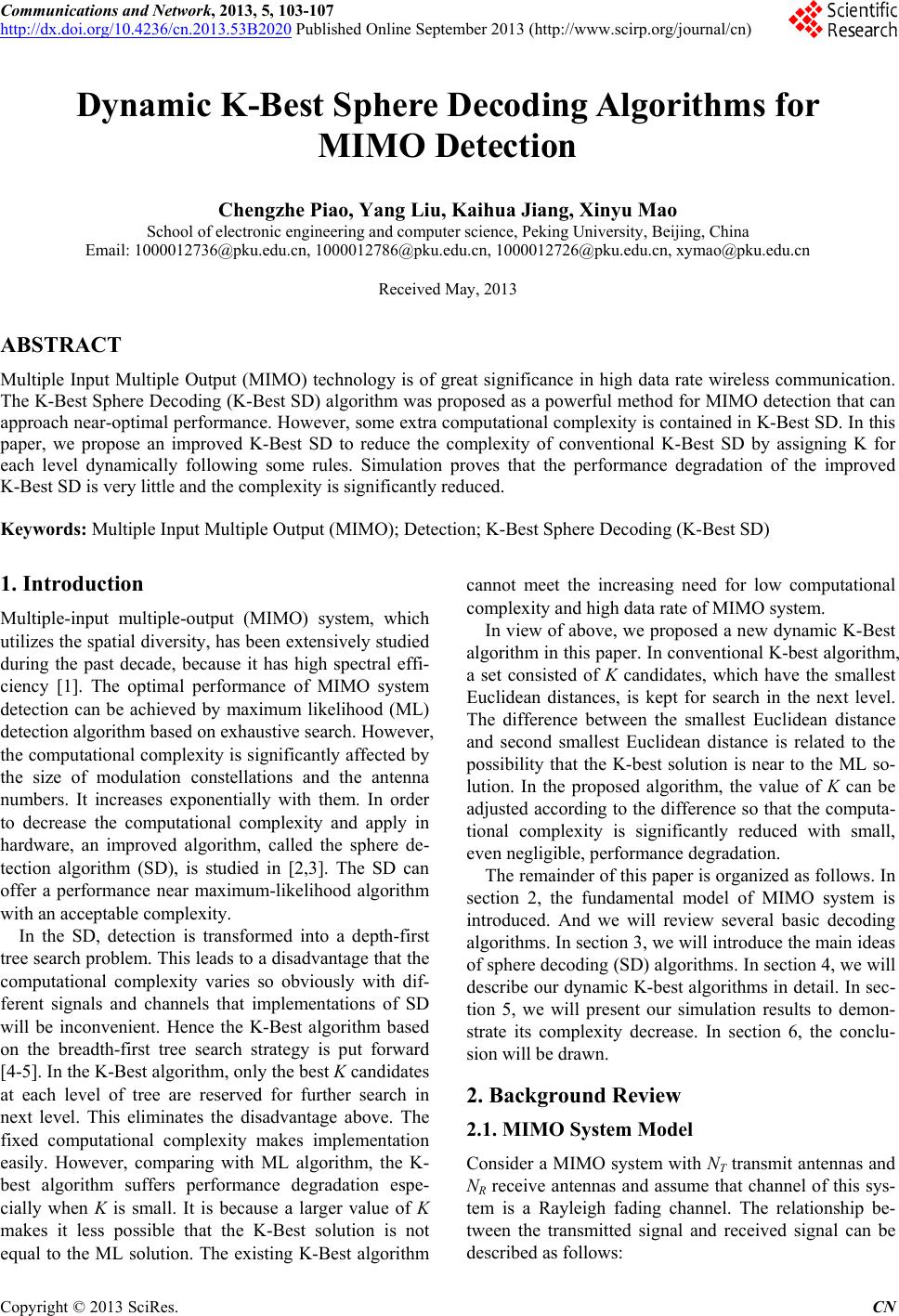
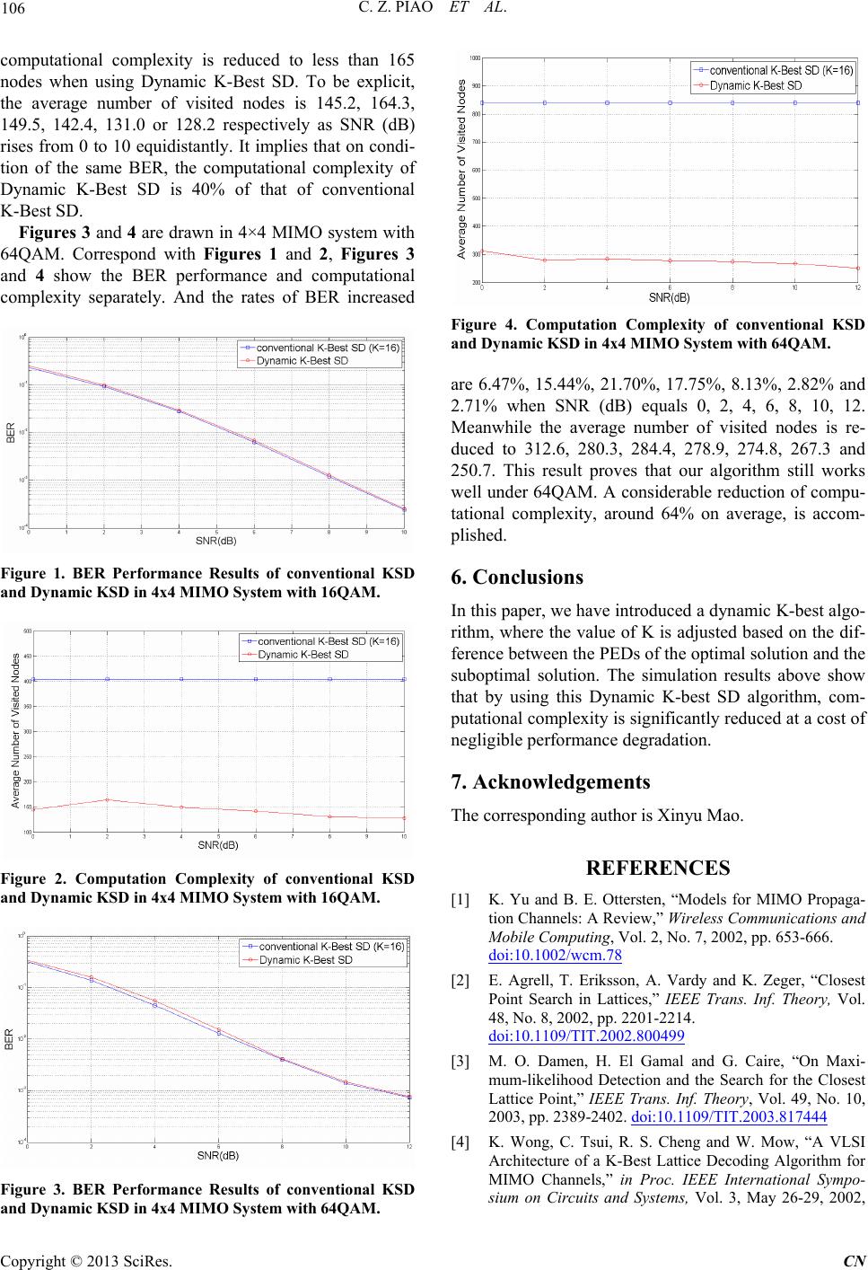
Figures 1 and 2 are drawn when 16QAM is applied.
Figure 1 shows the BER performance of the Dynamic
K-Best SD as well as the conventional K-Best SD. It is
obvious that in Figure 1 the interval between the two
curves is almost negligible. By selecting appropriate
threshold values of each level, the rates of BER increased
approximately are 8.94%, 8.06%, 6.44%, 9.09%, 8.96%
and 6.25% when SNR (dB) equals 0, 2, 4, 6, 8 and 10
respectively. All of the rates of BER increased by Dy-
namic K-Best SD are less than 10%, which means prac-
tically the deterioration of BER can be igno red.
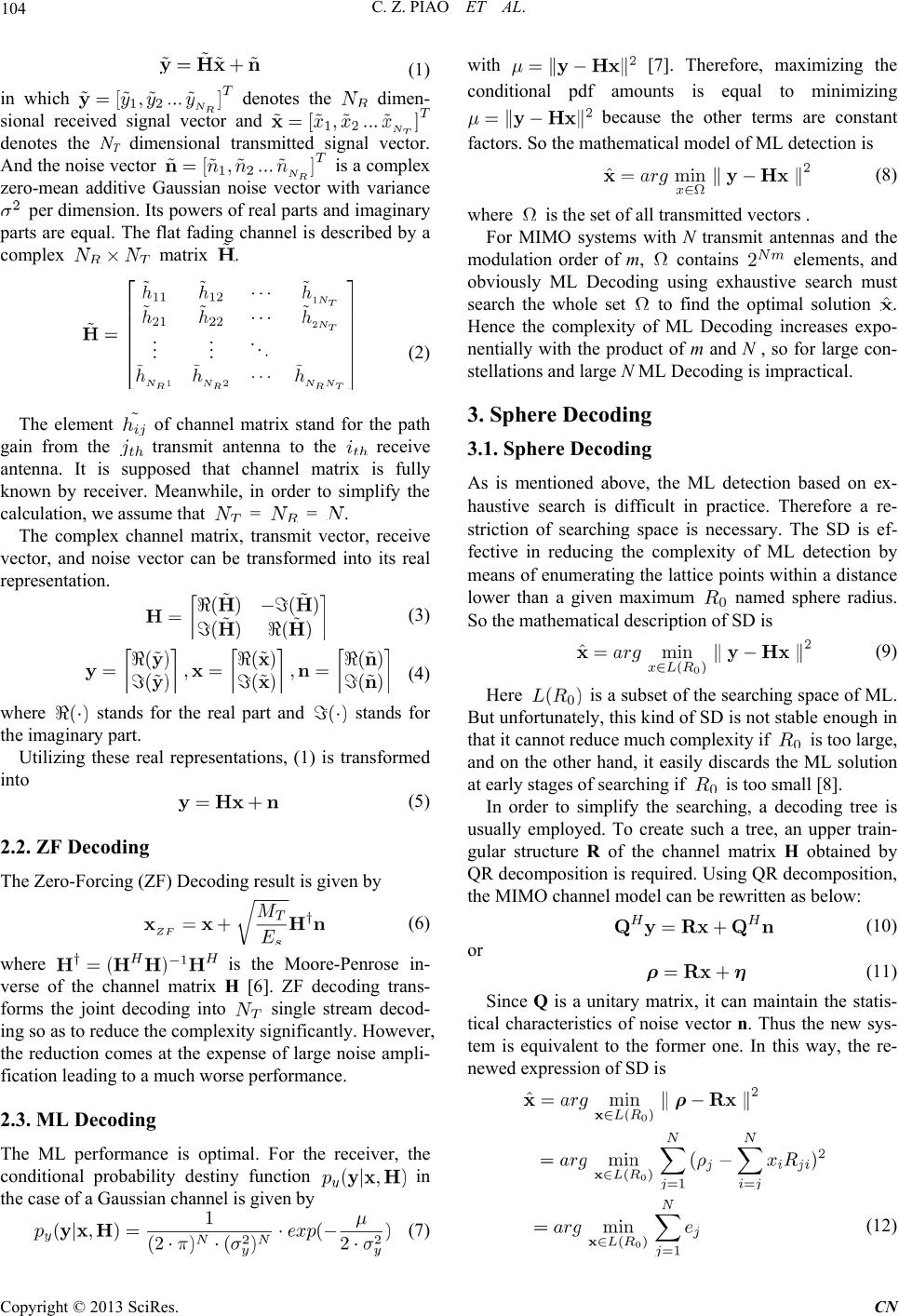
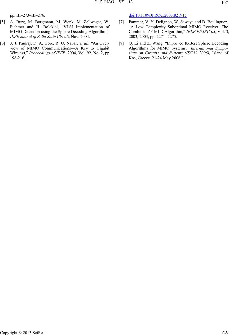
The computational complexity is characterized by the
average number of nodes visited in searching tree in this
paper. In Figure 2, it is concluded that compared with
404 nodes when using the conventional K-best SD, the

C. Z. PIAO ET AL.
106
computational complexity is reduced to less than 165
nodes when using Dynamic K-Best SD. To be explicit,
the average number of visited nodes is 145.2, 164.3,
149.5, 142.4, 131.0 or 128.2 respectively as SNR (dB)
rises from 0 to 10 equidistantly. It implies that on condi-
tion of the same BER, the computational complexity of
Dynamic K-Best SD is 40% of that of conventional
K-Best SD.
Figures 3 and 4 are drawn in 4×4 MIMO system with
64QAM. Correspond with Figures 1 and 2, Figures 3
and 4 show the BER performance and computational
complexity separately. And the rates of BER increased
Figure 1. BER Performance Results of conventional KSD
and Dynamic KSD in 4x4 MIMO System with 16QAM.
Figure 2. Computation Complexity of conventional KSD
and Dynamic KSD in 4x4 MIMO System with 16QAM.
Figure 3. BER Performance Results of conventional KSD
and Dynamic KSD in 4x4 MIMO System with 64QAM.
Figure 4. Computation Complexity of conventional KSD
and Dynamic KSD in 4x4 MIMO System with 64QAM.
are 6.47%, 15.44%, 21.70%, 17.75%, 8.13%, 2.82% and
2.71% when SNR (dB) equals 0, 2, 4, 6, 8, 10, 12.
Meanwhile the average number of visited nodes is re-
duced to 312.6, 280.3, 284.4, 278.9, 274.8, 267.3 and
250.7. This result proves that our algorithm still works
well under 6 4QAM. A considerable r eduction of compu-
tational complexity, around 64% on average, is accom-
plished.
6. Conclusions
In this paper, we have introduced a dynamic K-best algo-
rithm, where the value of K is adjusted based on the dif-
ference between the PEDs of the op timal solutio n and th e
suboptimal solution. The simulation results above show
that by using this Dynamic K-best SD algorithm, com-
putational complexity is significantly reduced at a cost of
negligible per f ormance degradati on.
7. Acknowledgements
The corresponding author is Xinyu Mao.
REFERENCES
[1] K. Yu and B. E. Ottersten, “Models for MIMO Propaga-
tion Channels: A Review,” Wireless Communications and
Mobile Computing, Vol. 2, No. 7, 2002, pp. 653-666.
doi:10.1002/wcm.78
[2] E. Agrell, T. Eriksson, A. Vardy and K. Zeger, “Closest
Point Search in Lattices,” IEEE Trans. Inf. Theory, Vol.
48, No. 8, 2002, pp. 2201-2214.
doi:10.1109/TIT.2002.800499
[3] M. O. Damen, H. El Gamal and G. Caire, “On Maxi-
mum-likelihood Detection and the Search for the Closest
Lattice Point,” IEEE Trans. Inf. Theory, Vol. 49, No. 10,
2003, pp. 2389-2402. doi:10.1109/TIT.2003.817444
[4] K. Wong, C. Tsui, R. S. Cheng and W. Mow, “A VLSI
Architecture of a K-Best Lattice Decoding Algorithm for
MIMO Channels,” in Proc. IEEE International Sympo-
sium on Circuits and Systems, Vol. 3, May 26-29, 2002,

C. Z. PIAO ET AL.
107
pp. III–273–III–276.
[5] A. Burg, M. Borgmann, M. Wenk, M. Zellweger, W.
Fichtner and H. Bolcklei, “VLSI Implementation of
MIMO Detection using the Sphere Decoding Algorithm,”
IEEE Jounal of Solid State Circuit, Nov. 2004.
[6] A J. Paulraj, D. A. Gore, R. U. Nabar, et al., “An Over-
view of MIMO Communications—A Key to Gigabit
Wireless,” Proceedings of IEEE, 2004, Vol. 92, No. 2, pp.
198-216.
doi:10.1109/JPROC.2003.821915
[7] Pammer, V. Y. Delignon, W. Sawaya and D. Boulinguez,
“A Low Complexity Suboptimal MIMO Receiver: The
Combined ZF-MLD Algorithm,” IEEE PIMRC’03, Vol. 3,
2003, 2003, pp. 2271 -2275.
[8] Q. Li and Z. Wang, “Improved K-Best Sphere Decoding
Algorithms for MIMO Systems,” International Sympo-
sium on Circuits and Systems (ISCAS 2006), Island of
Kos, Greece. 21-24 May 2006.L.