Paper Menu >>
Journal Menu >>
 Journal of Intelligent Learning Systems and Applications, 2011, 3, 17-25 doi:10.4236/jilsa.2011.31003 Published Online February 2011 (http://www.SciRP.org/journal/jilsa) Copyright © 2011 SciRes. JILSA 17 Function Approximation Using Robust Radial Basis Function Networks Oleg Rudenko, Oleksandr Bezsonov The Department of Computer Engineering and Control, Kharkov National University of Radio Electronics, Kharkiv, Ukraine. Email: o.bezsonov@gmail.com Received April 9th, 2010; revised July 20th, 2010; accepted August 4th, 2010 ABSTRACT Resistant training in radial basis function (RBF) networks is the topic of this paper. In this paper, one modification of Gauss-Newton training algorithm based on the theory of robust regression for dealing with outliers in the framework of function approximation, system identification and control is proposed. This modification combines the numerical ro- bustness of a particular class of non-quadratic estimators known as M-estimators in Statistics and dead-zone. The al- gorithms is tested on some examples, and the results show that the proposed algorithm not only eliminates the influence of the outliers but has better convergence rate then the standard Gauss-Newton algorithm. Keywords: Neural Network, Robust Training, Basis Function, Dead Zone 1. Introduction Function approximation involves estimating (approxi- mating) the underlying relationship from a given finite input-output data set yxf x (1) where 1M xR is an input vector; f is the arbi- trary nonlinear fun ction , unknown in the general case; is the unobserved disturbance with unknown characteris- tics; has been the fundamental problem for a variety of applications in system identification, pattern classifica- tion, data mining and signal reconstruction [1-4]. Feedforward neural networks such as multilayer per- ceptrons (MLP) have been widely used as an approach to function approximation since they provide a generic black-box functional representation and have been shown to be capable of approximating any continuous function defined on a compact set in N R with arbitrary accuracy [5-7]. It has been proved that a radial basis function network (RBF) can approximate arbitrarily well any multivariate continuous function on a compact domain if a sufficient number of ra dial basis functi on units are gi ven [8]. In contrast to MLPs, RBF networks use a localized re- presentation of information. The RBF network requires less computation time for the learning and more compact topology than MLP. The network can be co nfigured with one radial basis function centre at each training data point. Thus, the complexity of the network is of the same order as the dimensionality of the training data and the network has a poor generalization capability. The RBF decomposition of f x is 0 ˆ,, NT ii i f xwxrwxr (2) where 1N wR is a vector of linear weights, 1 N R is a vector of RBFs and r is a distance. An important advantage of RBFN from viewpoint of practitioners is, therefore, clear and understandable in- terpretation of the functionality of basis functions. The traditional RBF basis function is defined by Euc- lidian distance E ij rxt and Gaussian activation function by 22 exp 0.5 ji E xr , where i x is the input sample number i, j t is the center of j-th radial basis function (radii), is the standard deviation. If we use the Mahalanobis distance 1 T M ij ij rxtRxt where 1k ij Rr is weight matrix, M is the dimension of input vector i x , N is the number of neurons, for the RBF activation function we have 1 exp T jjjj x xtR xt (3) where j R is the covariance matrix. Geometrically j t represents the center and j R the shape of the j-th basis  Function Approximation Using Robust Radial Basis Function Networks Copyright © 2011 SciRes. JILSA 18 function. A hidden unit function can be represented as a hyper-ellipsoid in the N-dimensional space. All the network parameters (weights, centers and radii) may be determined using various learning algorithms have been used in order to find the most appropriate pa- rameters for the RBF decomposition. A network iteratively adjusts parameters of each node by minimizing some cost function which can be defined as an ensemble average errors. 1 1 ,, k i Fek ei k (4) where ,ei is a scalar loss function; ˆ , eiyifi represents the residual error be- tween the desired y i, and the actual network outputs, ˆ f i; i—indicates the index of the series; comprises all the unknown parameters of the network, 0111 11 11,1, 11,1, ,,,, , , ,,, ,,,,,, MMM T NNN NN MMM kcct trr ctt rr . The problem of neural network training (estimating ) which approximates the function (1) “well”, has essen- tially been tackled, based on the following two different assumptions [9]: (A1) The noise has some probabilistic and/or statistical properties. (A2) Regardless of the disturbance nature, a noise bound is available, i.e. 22 kk . Assumption (A1) leads to different stochastic training methods that are based on minimization of some loss function. Different choices of loss functions arise from various assumptions about the distribution of the noise in measurement. The most common loss function is the quadratic function corresponding to a Gaussian noise model with zero mean, and a standard deviation that does not depend on the inputs. The Gaussian loss function is used popularly as it has nice analytical properties. How- ever, one of the potential difficulties of the standard qua- dratic loss function is that it receives the large contribu- tions from outliers that have particularly large errors. The problems in the neural network training are that when the training data sets contain outliers, traditional supervised learning algorithms usually cannot come up acceptable performance. Since traditional training algorithms also adopt the least-square cost function (4), those algorithms are very sensitive to outliers. Techniques that attempt to solve these problems are referred to robust statistics [10,11]. In recent years, vari- ous robust learning algorithms based on M-estimation have been proposed to overcome the outlier’s problems [12-17]. The basic idea of M-estimators is to replace the quad- ratic function in the cost function (4) by the loss function so that effect of those outliers may be degraded. Traditional approaches of solving such a problem are to introduce a robust cost function (4), and then, a steep- est descent approach is applied. The idea of such an ap- proach is to identify outliers and then to reduce the effect of outliers directly. Alternative approaches have been formulated in a de- terministic framework based on Assumption (A2). In this context th e training prob lem is then to find a θ belonging to the class of models (2) for which the absolute value of the difference between the function (1) and model is smaller than k for all times k. Three different types of solutions to this problem have mainly been explored in literature. The first method is to formulate the estimation problem in a geometrical setting. Different proposals result from this approach but Fogel and Huang [18] proposed a minimal volume recursive algorithm (FHMV) which minimizes the size of an ellip- soid and was attractive for on-line estimation. The second alternative is to derive estimation algo- rithm for stability consideration together with the geo- metrical (ellipsoidal-outer-bounding algorithm by Lozano- Leal and Ortega) [19]. The third approach is to obtain estimation (training) algorithm from modifying the ex- ponentially weighted recursive least squares algorithm (EW-RLS) [9]. All these algorithms have a dead zone. The dead zone scheme guarantees convergence of the neural network training algorithm in the present of noise 22 kk . It should be noted that this dead zone may serve as value that limits the accuracy of the obtained solutions, i.e. determines its acceptable inaccuracy. The proposed method combines the numerical robust- ness of a particular class of non-quadratic M-estimators and dead-zone. 2. Robust Gauss-Newton Training Algorithm The estimation ˆ is the solution of the following set of equations 1 , 1,0 k i jj Fe ei ei k (5) where , ,,, , ei eiei ei ei is the influence function and ,ei is the weight function. For quadratic function ,ei in the maximum likehood estimation case (5) has a closed form solution, the sample mean. The sample mean is substantially af-  Function Approximation Using Robust Radial Basis Function Networks Copyright © 2011 SciRes. JILSA 19 fected by the presence of outliers. For many non-quadratic loss functions, the Equation (5) does not have closed form solution, but can be solved by the some iterative or recursive m ethods. The minimization of the criterion (4) can therefore be performed using Gauss-Newton algorithm. ˆ 1 ˆˆ 1ˆˆ 11 T Pkfkek kk ek fkPkfk (6) 1 ˆˆ 11 ˆˆ 11 T T Pk Pk Pkfk fkPkek ekf kPkf k (7) where 01111 1,1 1,2 11 1 1,,1,1 , ˆˆˆˆˆ ˆ,,,,,, ˆ ˆ ˆˆˆ ˆ ,, ,, , , ,, T NN NN MMM MM fk fk fk fk fk fk cctrr fkfkfk fk fkfk rr ctrr 0 ˆ1 fk c ˆ,, iii i fk x tR c ˆA i ii fk A ce tt ˆA i ij ij mm fk A ce rr with 1 T j j A xtR xt . The initial value of the matrix 0P is chosen as in the recursive MLS (RMLS), i.e. 0PI , where 1 , and the initial dimension of the identity matrix I is given as SS, where 2 11SMM is number of adjustable parameters of a network contain- ing 1 neuron. Because after the introduction into the network a new n-th neuron the dimension of the Pk increases, the values of elements in matrix Pk are reset and initialized again, then S becomes equal to 2 11SnMM , where n—the current number of neurons in the network. The influence function e measures the influence of a datum on the value of the parameter estimate. For example, for the least-squares with 2 0.5ee , the influence function is ee , that is, the influence of a datum on the estimate increases linearly with the size of its error and without bound, which confirms the non- robustness of the least-squares estimate. Huber proposed a robust estimator so-called an M-es- timator, M for maximum likelihood. M-estimator is the solution of (5) where different non-quadratic loss func- tion ,ei are used. Following Huber [10], a distribution of the noise con- taminated by outliers expressed by a mixture of two probability density functions 0 1pxp xqx (8) where 0 px is the density of basic distribution of a measurement noise; qx is the density of a distribu- tion of outliers; 0,1 is the probability of occurring a large error. Even if the basic 0 px and contaminating qx distributions are Gaussian with zero mean and variances 2 1 and 2 2 , 22 12 hence, than optimal for the Gaussian distribution estimations (6)-(7), obtained by choosing 2 0.5ee , will be unstable. The density distribution * p for —contaminated pro- bability distributions (8), which gives the minimum Fisher information, contains a central region 0 1pp and tails with exponentially decreasing density 0 p x ce . Usage of these distributions allowed to ob- tain nonlinear robust Maximum likelihood estimates, that are workable for almost all the noise distributions. This algorithm combines the conventional least mean square (LMS) if 2 1 3ek and least absolute devia- tion (LAD) if 2 1 3ek stochastic gradient algo- rithms and called the mixed-norm LMS algorithm [10,20,21]. On the other hand, the choice of loss function, differ- ent from the quadratic, ensures the robustness of esti- mates, i.e. their workability for almost all distributions of noises. Currently, there are many such functions e , however, keeping in mind that ek ek is used in the learning algorithm (6)-(7) it is advisable to choose such functions ek , which have nonzero second derivatives. As these functions can be taken, for example [22,23], 2 12 ek Fekc (9) 2lncosh ek Fek cc (10) 2 322 ek Fek cek (11) graphs of which are shown in Table 1. It should be noted that in case of using functionals as (9) and (10) a problem of the selection (evaluation) of parameter с (in Table 1 shapes of the functionals with c = 5 are shown) arises. The standard deviations 2 1 and 2 2 in (8) are usually unknown and must be estimated and they can be  Current Distortion Evaluation in Traction 4Q Constant Switching Frequency Converters Copyright © 2011 SciRes. JILSA 20 Table 1. Graphs of functions (9)-(11), their first and second derivatives and weight functions. F ek ek ek ek 1 F ek 2 F ek 3 F ek taken into account in the learning algorithm. If 2 1 and 2 2 do not change over time, this evaluation can be car- ried out by stochastic approximation: 222 11 1 2 11 2 1 1 ˆˆ 11 ˆˆ for3 1 ˆ1 otherwise kekk lk k ekk k (12) 222 22 2 2 21 2 2 1 ˆˆ 11 ˆˆ for3 1 ˆ1 otherwise kekk lk k ekk k where 12 lkk l k 1 2 2 ˆ 0 31 11 otherwise for ekk lk lk The total variance of noise, calculated as 2 11 2 2 2 ˆˆ for31 ˆ otherwise k ekk kk (13) can be used for normalizing the selected functional *2 2 , ,, ek ek (14) It should be noted that as estimation of the parameter с in the functionals (9) and (10) 3 can be used. 3. Modification of Robust Gauss-Newton Algorithm with Dead Zone Dead zone, which determines the degree of permissible errors, can be set as follows: ** * 1* for ,0 for ek ek ek ek (15) and ** ** 2 ** for ,0 for for . ek ek ek ek ek ek (16) The forms of functions (12) and (13) are shown in the Table 2 (columns 2 and 3, respectively). In this case, the robust Gauss-Newton algorithm takes the form 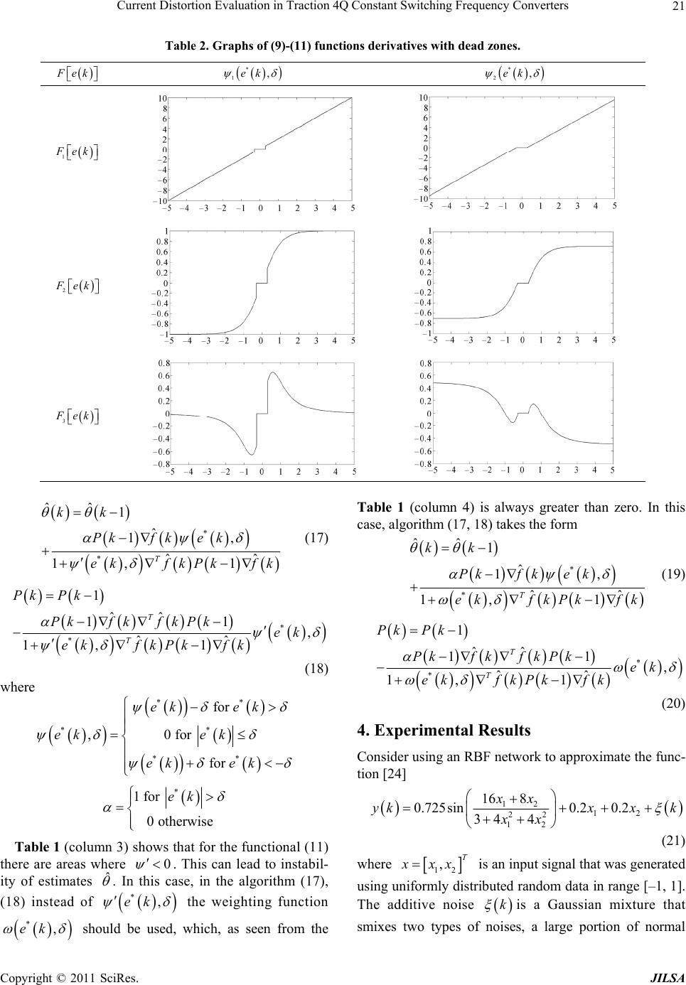 Current Distortion Evaluation in Traction 4Q Constant Switching Frequency Converters Copyright © 2011 SciRes. JILSA 21 Table 2. Graphs of (9)-(11) functions derivatives with dead zones. F ek * 1,ek * 2,ek 1 F ek 2 F ek 3 F ek * * ˆˆ 1 ˆ 1, ˆˆ 1,1 T kk Pkf kek e kfkPkfk (17) * * 1 ˆˆ 11 , ˆˆ 1,1 T T Pk Pk Pkf kfkPkek e kfkPkfk (18) where ** ** ** for ,0 for for ek ek ek ek ek ek * 1 for 0 otherwise ek Table 1 (column 3) shows that for the functional (11) there are areas where 0 . This can lead to instabil- ity of estimates ˆ . In this case, in the algorithm (17), (18) instead of *,ek the weighting function *,ek should be used, which, as seen from the Table 1 (column 4) is always greater than zero. In this case, algorithm (17, 18) takes the form * * ˆˆ 1 ˆ 1, ˆˆ 1, 1 T kk Pkf kek ekfkPkfk (19) * * 1 ˆˆ 11 , ˆˆ 1, 1 T T Pk Pk Pkfk fkPkek e kfkPkfk (20) 4. Experimental Results Consider using an RBF network to approximate the func- tion [24] 12 12 22 12 16 8 0.725sin0.2 0.2 34 4 xx ykxx k xx (21) where 12 ,T x xx is an input signal that was generated using uniformly distributed random data in range [–1, 1]. The additive noise k is a Gaussian mixture that smixes two types of noises, a large portion of normal 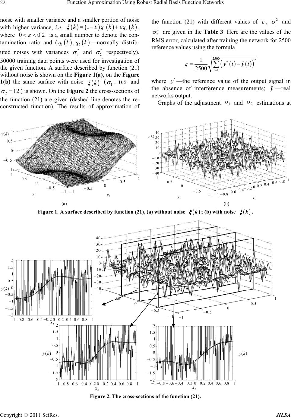 Function Approximation Using Robust Radial Basis Function Networks Copyright © 2011 SciRes. JILSA 22 noise with smaller variance and a smaller portion of noise with higher variance, i.e. 12 1kqkqk , where 00.2 is a small number to denote the con- tamination ratio and ( 1 qk, 2 qk —normally distrib- uted noises with variances 2 1 and 2 2 respectively). 50000 training data points were used for investigation of the given function. A surface described by function (21) without noise is shown on the Figure 1(a), on the Figure 1(b) the same surface with noise k (10.6 and 212 ) is shown. On the Figure 2 the cross-sections of the function (21) are given (dashed line denotes the re- constructed function). The results of approximation of the function (21) with different values of , 2 1 and 2 2 are given in the Table 3. Here are the values of the RMS error, calculated after train ing the networ k for 2500 reference values using the formula 2500 2 * 1 1ˆ 2500 i yi yi where * y —the reference value of the output signal in the absence of interference measurements; ˆ y—real networks output. Graphs of the adjustment 1 and 2 estimations at (a) (b) Figure 1. A surface described by function (21), (a) without noise k; (b) with noise k. Figure 2. The cross-sections of the function (21).  Function Approximation Using Robust Radial Basis Function Networks Copyright © 2011 SciRes. JILSA 23 (a) (b) Figure 3. Results of the estimation 10.6 and 212 with 0.2 . Table 3. The results of function (21) approximation. Table 4. Estimations of 1 , 2 and N. Given parameters Estimations 1 ref 2 ref Real number of outliers 1 est 2 est Estimated number of outliers N 0.0 0 0 0 - - - 0.1 0.6 3 5061 0.6369 4.0902 4758 6 5008 0.6166 6.7468 4984 12 4991 0.6073 12.5611 4969 0.2 0.6 3 10013 0.7351 4.3658 9957 6 10020 0.6151 6.8815 9897 12 10111 0.6220 12.8381 10005 each step of training the network are shown in Figure 3. Estimations of 1 , 2 and number of outliers are given in Table 4. As seen from the simulation results, the algorithm (12) gives reasonably accurate estimates of 2 1 and 2 2 (assuming 22 12 ) that are used in the normalization of the loss function, which ensures high accuracy of ap- Given parameters 2 2 ek Fekc ln coshek Fekcc 2 32 1 ek Fek ek (with a weight function) 1 ref 2 ref Number of outliers without dead zone With dead zone (15) with dead zone (16) without dead zone with dead zone (15) with dead zone (16) without dead zone with dead zone (15) with dead zone (16) 0.0 0 0 0 0.6286 - - - - - - - - 0.1 0.6 3 5061 1.5252 2.7339 2.6047 1.5556 2.4468 2.3937 2.0836 2.8747 2.8137 6 5008 1.6415 2.4909 2.4697 1.6553 2.2052 2.2047 1.8936 2.7882 2.7199 12 4991 1.9389 1.9634 1.9491 1.7256 1.7386 1.7379 1.6365 2.3665 2.3088 0.2 0.6 3 10013 1.6497 2.1061 2.0698 2.3438 3.0111 2.9940 2.9080 2.9365 2.9198 6 10020 2.0402 2.1209 2.0813 2.2875 2.4361 2.4113 2.2054 2.7103 2.5998 12 10111 1.9863 2.2117 2.1887 2.3682 2.7750 2.7217 2.5152 2.7012 2.6260  Function Approximation Using Robust Radial Basis Function Networks Copyright © 2011 SciRes. JILSA 24 proximation of very noisy nonlinear functions. Also it should be noted that the usage of dead zones has reduced training time by about 20%. 5. Conclusions This paper proposes a resistant radial function network on-line training algorithm based on the theory of robust regression for dealing with outliers in the framework of function approximation. The proposed algorith m minimizes an M-estimate cost functions instead of the conventional mean square error and represents one modification of recursive Gauss- Newton algorithm with dead-zone. These dead zone may serve as value that limits the accuracy of the obtained solutions. Utilization of dead zones can decrease training time of the network. If the distribution of the noise contaminated by outliers expressed by a mixture of two Gaussian distributions with unknown standard deviations 2 1 and 2 2 , 22 12 these can be estimated and taken into account in the training algorithm. It is an efficient algorithm for practical using in inves- tigation of real nonlinear systems. It is expedient to develop this approach further and to investigate other robust cost functions and training algorithms such as Levenberg-Marquardt algorithm. REFERENCES [1] B. Kosko, “Neural Network for Signal Processing,” Pren- tice-Hall Inc., New York, 1992. [2] S. Haykin, “Neural Networks. A Comprehensive Founda- tion,” 2nd Edition, Prentice Hall Inc., New York, 1999. [3] C. M. Bishop, “Neural Network for Pattern Recognition,” Clarendon Press, Oxford, 1995. [4] H. Wang, G. P. Liu, C. J. Harris and M. Brown, “Ad- vanced Adaptive Control,” Pergamon, Oxford, 1995. [5] R. Hecht-Nielsen, “Kolmogorov’s Mapping Neural Net- works Existence Theorem,” First IEEE International Conference on Neural Networks, San Diego, Vol. 3, 1987, pp. 11-14. [6] G. Cybenko, “Approximation by Superpositions of a Sigmoidal Function,” Mathematics of Control, Signals and Systems, Vol. 2, No. 4, 1989, pp. 303-314. doi:10. 1007/BF02551274 [7] T. Poggio and F. Girosi, “Networks for Approximation and Learning,” Proceeding of the IEEE, Vol. 78, No. 9, 1990, pp. 1481-1497. doi:10.1109/5.58326 [8] J. Park and I. W. Sandberg, “Universal Approximation Using Radial-Basis-Function Network,” Neural Compu- tation, Vol. 3, No. 2, 1991, pp. 246-257. doi:10.1162/ neco.1991.3.2.246 [9] C. C. de Wit and J. Carrillo, “A Modified EW-RLS Algo- rithms for Systems with Bounded Disturbances,” Auto- matica, Vol. 26, No. 3, 1990, pp. 599-606. doi:10.1016/ 0005-1098(90)90032-D [10] P. J. Huber, “Robust Statistics,” John Wiley, New York, 1981. doi:10.1002/0471725250 [11] R. E. Frank, M. Hampel, M. Rohchetti and W. A. Stanel, “Robust Statistics: The Approach Based on Influence Functions,” John Wiley & Sons Inc., Hoboken, 1986. [12] C. C. Chang, J. T. Jeng and P. T. Lin, “Annealing Robust Radial Basis Function Networks for Function Approxi- mation with Outliers,” Neurocomputing, Vol. 56, 2004, pp. 123-139. doi:10.1016/S0925-2312(03)00436-3 [13] S.-C. Chan and Y.-X. Zou, “A Recursive Least M-Esimate Algorithm for Robust Filtering in Impulsive Noise: Fast Algorithm and Convergence Perf ormance Analysis,” IEEE Transactions on Signal Processing, Vol. 52, No. 4, 2004, pp. 975-991. doi:10.1109/TSP.2004.823496 [14] D. S. Pham and A. M. Zoubir, “A Sequential Algorithm for Robust Parameter Estimation,” IEEE Signal Proce- ssing Letters, Vol. 12, No. 1, 2005, pp. 21-24. doi:10.11 09/LSP.2004.839689 [15] J. Ni and Q. Soug, “Pruning Based Robust Backpropaga- tion Training Algorithm for RBF Network Training Con- troller,” Intelligent and Robotic Systems, Vol. 48, No. 3, 2007, pp. 375-396. doi:10.1007/s10846-006-9093-x [16] G. Deng, “Sequential and Adaptive Learning Algorithms for M-Estimation,” EURASIP Journal on Advances in Signal Processing, Vol. 2008, 2008, ID 459586. [17] C.-C. Lee, Y.-C. Chiang, C.-Y. Shin and C.-L. Tsai, “Noisy Time Series Prediction Using M-Estimator Based Robust Radial Basis Function Network with Growing and Pruning Techniques,” Expert Systems with Applications, Vol. 36, No. 3, 2008, pp. 4717-4724. doi:10.1016/j.eswa. 2008.06.017 [18] E. Fogel and Y. E. Huang, “On the Value of Information in System Identification Bounded-Noise Case,” Auto- matica, Vol. 18, No. 2, 1982, pp. 229-238. doi:10.1016/ 0005-1098(82)90110-8 [19] R. Lozano-Leal and R. Ortega, “Reformulation of the Parameter Identification Problem for Systems with Bounded Disturbances,” Automatica, Vol. 23, No. 2, 1987, pp. 247-251. doi:10.1016/0005-1098(87)90100-2 [20] J. Chambers and A. Alvonitis, “A Robust Mixed-Norm Adaptive Filter Algorithm,” IEEE Signal Proceeding Letters, Vol. 4, No. 22, 1997, pp. 46-48. doi:10.1109/97. 554469 [21] Y. Zou, S. C. Chan and T. S. Ng, “A Recursive Least M-Estimate (RLM) Adaptive Filter for Robust Filtering in Impulse Noise,” IEEE Signal Proceeding Letters, Vol. 7, No. 11, 2000, pp. 324-326. doi:10.1109/97.873571 [22] P. W. Holland and R. E. Welsh, “Robust Regression Us- ing Iteratively Reweighted Least Squares,” Communica- tions in Statistics-Theory Mathematics, Vol. A6, 1977, pp. 813-827. doi:10.1080/03610927708827533 [23] S. Geman and D. McClure, “Statistical Methods for To- mographic Image Reconstruction,” Bulletin of the Inter-  Function Approximation Using Robust Radial Basis Function Networks Copyright © 2011 SciRes. JILSA 25 national Statistical Institut, Vol. L2, No. 4, 1987, pp. 4-5. [24] K. S. Narendra and K. Parthasarathy, “Identification and Control of Dynamical Systems Using Neural Networks,” IEEE Transactions on Neural Networks, Vol. 1, No. 1, 1990, pp. 4-26. doi:10.1109/72.80202 |

