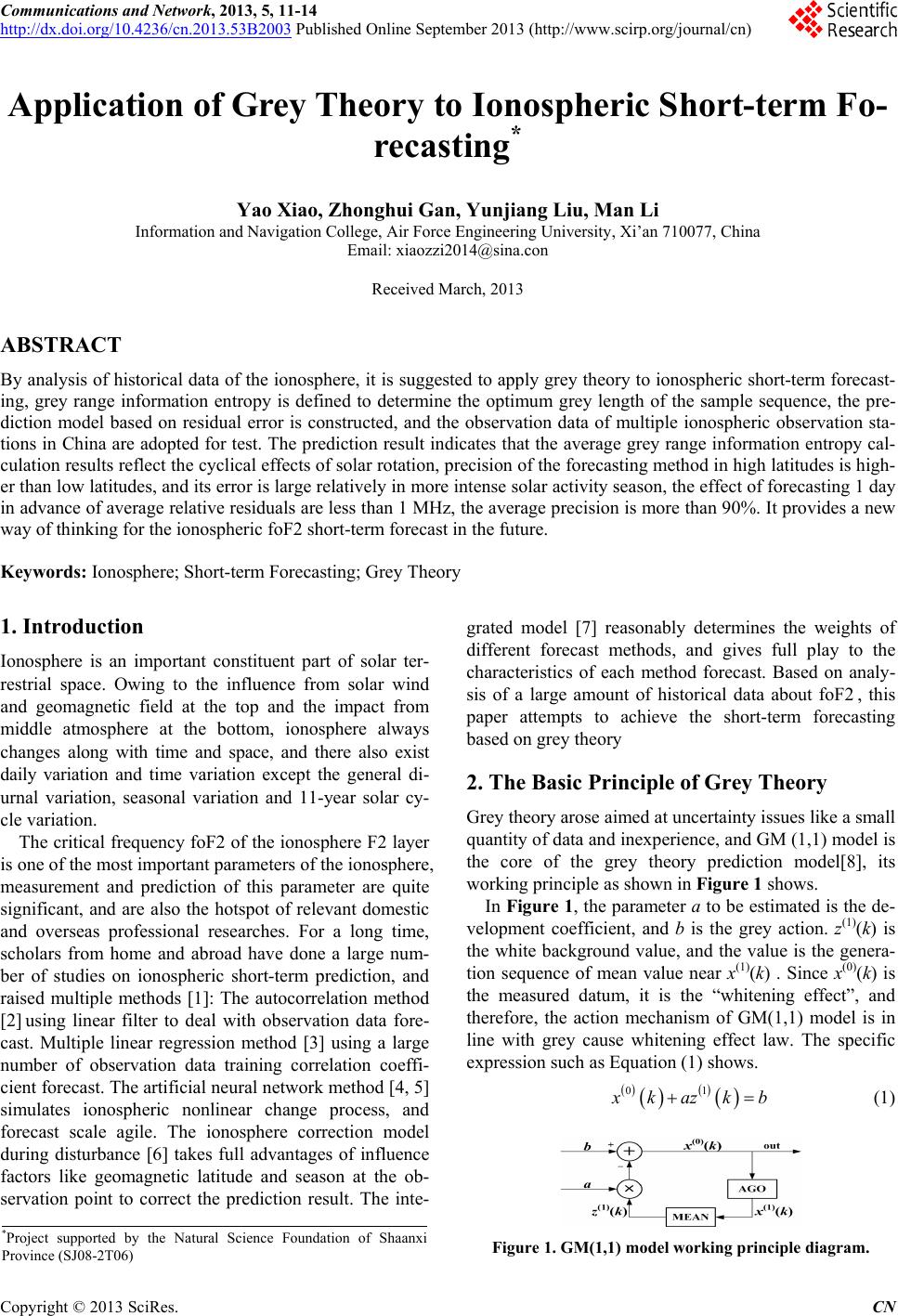Communications and Network, 2013, 5, 11-14
http://dx.doi.org/10.4236/cn.2013.53B2003 Published Online September 2013 (http://www.scirp.org/journal/cn)
Application of Grey Theory to Ionospheric Short-term Fo-
recasting*
Yao Xiao, Zhonghui Gan, Yunjiang Liu, Man Li
Information and Navigation College, Air Force Engineering University, Xi’an 710077, China
Received March, 2013
ABSTRACT
By analysis of historical data of the ionosphere, it is suggested to apply grey theory to ionospheric short-term forecast-
ing, grey range information entropy is defined to determine the optimum grey length of the sample sequence, the pre-
diction model based on residual error is constructed, and the observation data of multiple ionospheric observation sta-
tions in China are adopted for test. The pred iction result indicates that the average grey range information entropy cal-
culation results reflect the cyclical effects of solar rotatio n, precision of the forecastin g method in high latitude s is high-
er than low latitudes, and its error is large relatively in more intense solar activity season, the effect of forecasting 1 day
in advance of average relative residu als are less than 1 MHz, the average precision is more than 90%. It provides a new
way of thinking for the ionospheric foF2 short-term forecast in the future.
Keywords: Ionosphere; Short-term Forecasting; Grey Theory
1. Introduction
Ionosphere is an important constituent part of solar ter-
restrial space. Owing to the influence from solar wind
and geomagnetic field at the top and the impact from
middle atmosphere at the bottom, ionosphere always
changes along with time and space, and there also exist
daily variation and time variation except the general di-
urnal variation, seasonal variation and 11-year solar cy-
cle variation.
The critical frequency foF2 of the ionosphere F2 layer
is one of the most important parameters of the ionosphere,
measurement and prediction of this parameter are quite
significant, and are also the hotspot of relevant domestic
and overseas professional researches. For a long time,
scholars from home and abroad have done a large num-
ber of studies on ionospheric short-term prediction, and
raised multiple methods [1]: The autocorrelation method
[2] using linear filter to deal with observation data fore-
cast. Multiple linear regression method [3] using a large
number of observation data training correlation coeffi-
cient forecast. The artificial neural network method [4, 5]
simulates ionospheric nonlinear change process, and
forecast scale agile. The ionosphere correction model
during disturbance [6] takes full advantages of influence
factors like geomagnetic latitude and season at the ob-
servation point to correct the prediction result. The inte-
grated model [7] reasonably determines the weights of
different forecast methods, and gives full play to the
characteristics of each method forecast. Based on analy-
sis of a large amount of historical data about foF2 , this
paper attempts to achieve the short-term forecasting
based on grey theory
2. The Basic Principle of Grey Theory
Grey theory arose aimed at uncertainty issues like a small
quantity of data and inexperience, and GM (1,1) model is
the core of the grey theory prediction model[8], its
working principle as shown in Figure 1 shows.
In Figure 1, the parameter a to be estimated is the de-
velopment coefficient, and b is the grey action. z(1)(k) is
the white background value, and the value is the genera-
tion sequence of mean value near x(1)(k) . Since x(0)(k) is
the measured datum, it is the “whitening effect”, and
therefore, the action mechanism of GM(1,1) model is in
line with grey cause whitening effect law. The specific
expression such as Equation (1) shows.




01
x
kazkb

 (1)
*Project supported by the Natural Science Foundation ofShaanxi
Province (SJ08-2T 0 6 ) Figure 1. GM(1,1) model working principle diagram.
C
opyright © 2013 SciRes. CN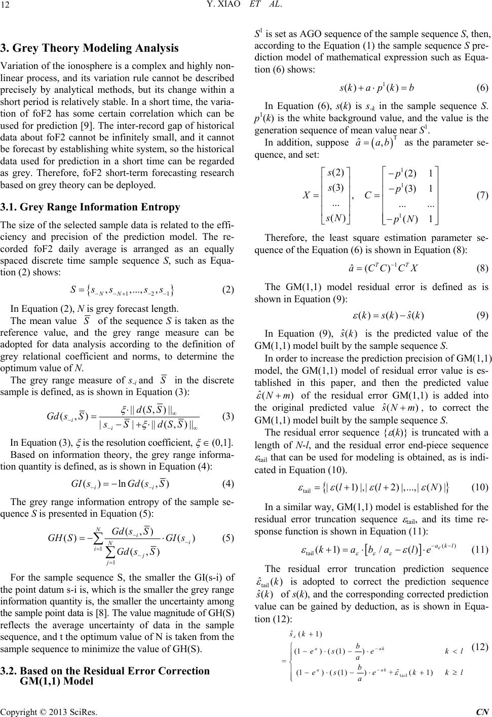

Y. XIAO ET AL.
12
3. Grey Theory Modeling Analysis
Variation of the ionosphere is a complex and highly non-
linear process, and its variation rule cannot be described
precisely by analytical methods, but its change within a
short period is relatively stable. In a short time, the varia-
tion of foF2 has some certain correlation which can be
used for prediction [9]. The inter-record gap of historical
data about foF2 cannot be infinitely small, and it cannot
be forecast by establishing white system, so the historical
data used for prediction in a short time can be regarded
as grey. Therefore, foF2 short-term forecasting research
based on grey theory can be deployed.
3.1. Grey Range Information Entropy
The size of the selected sample data is related to th e effi-
ciency and precision of the prediction model. The re-
corded foF2 daily average is arranged as an equally
spaced discrete time sample sequence S, such as Equa-
tion (2) sh ows:

121
,,..., ,
NN
Sss ss
 
 (2)
In Equation (2), N is grey forecast length.
The mean value S of the sequence S is taken as the
reference value, and the grey range measure can be
adopted for data analysis according to the definition of
grey relational coefficient and norms, to determine the
optimum value of N.
The grey range measure of s-i and S in the discrete
sample is defined, as is shown in Equation (3):
||(,)||
(,)||||(,)
ii
dSS
Gd sSsS dSS






 ||

(3)
In Equation (3),
 is the resolution coefficient,   (0,1] .
Based on information theory, the grey range informa-
tion quantity is defined, as is shown in Equation (4):
()ln(,)
i
GI sGd sS

 i (4)
The grey range information entropy of the sample se-
quence S is presented in Equation (5):
1
1
(,)
()( )
(,)
Nii
N
ij
j
Gd sS
GH SGI s
Gd sS



 
 (5)
For the sample sequence S, the smaller the GI(s-i) of
the point datum s-i is, which is the smaller the grey range
information quantity is, the smaller the uncertainty a mong
the sample point data is [8 ]. The value magnitud e of GH(S)
reflects the average uncertainty of data in the sample
sequence, and t the optimum value of N is taken from the
sample sequence to minimize the value of GH(S).
3.2. Based on the Residual Error Correction
GM(1,1) Model
S1 is set as AGO sequence of the sample sequence S, then,
according to the Equation (1) the sample sequence S pre-
diction model of mathematical expression such as Equa-
tion (6) shows:
1
() ()
s
kapkb

 (6)
In Equation (6), s(k) is s-k in the sample sequence S.
p1(k) is the white background value, and the value is the
generation sequence of mean value near S1.
In addition, suppose as the parameter se-
quence, and set:

T
ˆ,
aab
1
1
1
(2) (2) 1
(3) (3) 1
,
... ... ...
() ()1
sp
sp
XC
sN pN

  
 




 
 

 


(7)
Therefore, the least square estimation parameter se-
quence of the Equation (6) is shown in Equation (8):
1
ˆ()
TT
aCCCX

 (8)
The GM(1,1) model residual error is defined as is
shown in Equation (9):
ˆ ()() ()ksksk

 (9)
In Equation (9), ˆ()
s
k is the predicted value of the
GM(1,1) model built by the sample sequence S.
In order to increase the prediction precision of GM(1,1)
model, the GM(1,1) model of residual error value is es-
tablished in this paper, and then the predicted value
ˆ(Nm)


of the residual error GM(1,1) is added into
the original predicted value ˆ()
s
Nm, to correct the
GM(1,1) model built by the sample sequence S.
The residual error sequence {
 (k)} is truncated with a
length of N-l, and the residual error end-piece sequence

tail that can be used for modeling is obtained, as is indi-
cated in Equation (10).


tail |(1)|,|(2) |,...,|() |ll N
    (10)
In a similar way, GM(1,1) model is established for the
residual error truncation sequence 
tail, and its time re-
sponse function is shown in Equation (11):


()
tail (1)/()akl
kabale




  (11)
The residual error truncation prediction sequence
tail
ˆ()k

is adopted to correct the prediction sequence
ˆ()
s
k of s(k), and th e corresponding corrected prediction
value can be gained by deduction, as is shown in Equa-
tion (12):
tail
ˆ (1)
(1)((1))
=ˆ
(1)( (1))+(1)
aak
aak
sk
b
es ek
a
b
esek k
a





l
l

 





 


(12)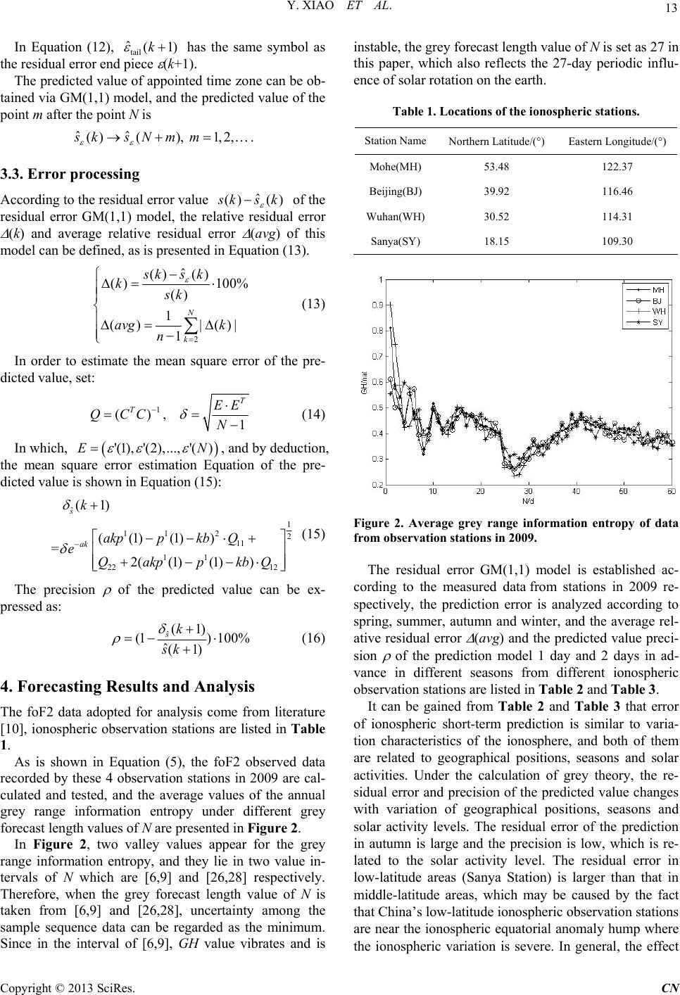

Y. XIAO ET AL. 13
In Equation (12), tail
ˆ(1k)

 has the same symbol as
the residual error end piece  (k+1).
The predicted value of appointed time zone can be ob-
tained via GM(1,1) model, and the predicted value of the
point m after the point N is
ˆˆ ()(), 1,2,sksN m m

 .
3.3. Error processing
According to the residual error value ˆ
() ()
s
ksk

 of the
residual error GM(1,1) model, the relative residual error
 (k) and average relative residual error  (avg) of this
model can be defined, as is presented in Equation (13).
2
ˆ () ()
( )100%
()
1
() |()|
1
N
k
sks k
ksk
avg k
n



 



 


(13)
In order to estimate the mean square error of the pre-
dicted value, set:
1
(),1
T
TEE
QCC N 


 (14)
In which, , and by deduction,
the mean square error estimation Equation of the pre-
dicted value is shown in Equation (15):

'(1), '(2),..., '()E   

N
ˆ
1
11 22
11
11
22 12
(1)
((1)(1))
=2( (1)(1) )
s
ak
k
akppkb Q
eQakppkbQ













(15)
The precision  of the predicted value can be ex-
pressed as:
ˆ(1)
(1) 100%
ˆ(1)
sk
sk



 
 (16)
4. Forecasting Results and Analysis
The foF2 data adopted for analysis come from literature
[10], ionospheric observation stations are listed in Table
1. As is shown in Equation (5), the foF2 observed data
recorded by these 4 observation stations in 2009 are cal-
culated and tested, and the average values of the annual
grey range information entropy under different grey
forecast length values of N are presented in Figure 2.
In Figure 2, two valley values appear for the grey
range information entropy, and they lie in two value in-
tervals of N which are [6,9] and [26,28] respectively.
Therefore, when the grey forecast length value of N is
taken from [6,9] and [26,28], uncertainty among the
sample sequence data can be regarded as the minimum.
Since in the interval of [6,9], GH value vibrates and is
instable, the grey forecast length value of N is set as 27 in
this paper, which also reflects the 27-day periodic influ-
ence of solar rotation on the earth.
Table 1. Locations of the ionospheric stations.
Station NameNorthern Latitude/() Eastern Longitude/()
Mohe(MH) 53.48 122.37
Beijing(BJ) 39.92 116.46
Wuhan(WH) 30.52 114.31
Sanya(SY) 18.15 109.30
Figure 2. Average grey range information entropy of data
from observation stations in 2009.
The residual error GM(1,1) model is established ac-
cording to the measured data from stations in 2009 re-
spectively, the prediction error is analyzed according to
spring, summer, autumn and winter, and the average rel-
ative residual error
 (avg) and the predicted value preci-
sion
 of the prediction model 1 day and 2 days in ad-
vance in different seasons from different ionospheric
observation stations are listed in Table 2 and Table 3.
It can be gained from Table 2 and Table 3 that error
of ionospheric short-term prediction is similar to varia-
tion characteristics of the ionosphere, and both of them
are related to geographical positions, seasons and solar
activities. Under the calculation of grey theory, the re-
sidual error and precision of the predicted value changes
with variation of geographical positions, seasons and
solar activity levels. The residual error of the prediction
in autumn is large and the precision is low, which is re-
lated to the solar activity level. The residual error in
low-latitude areas (Sanya Station) is larger than that in
middle-latitude areas, which may be caused by the fact
that China’s low- latitud e ionospher ic ob servatio n statio ns
are near the ionospheric equatorial anomaly hump where
the ionospheric variation is severe. In general, the effect

Y. XIAO ET AL.
14
Table 2. The
 (avg) of the predicted value in different seasons from stations / MHz.
One day in advance forecast Two days in advance forecast
Station Name Spring Summer Autumn Winter Spring Summer Autumn Winter
MH 0.39 0.24 0.43 0.41 1.52 1.47 2.05 1.93
BJ 0.13 0.20 0.41 0.33 1.68 1.51 2.15 1.83
WH 0.62 0.53 0.66 0.61 1.89 1.93 2.70 2.22
SY 0.76 0.87 0.94 0.82 2.06 2.28 2.82 2.47
Table 3. The predicted value precision
 in different seasons from stations / %.
One day in advance forecast Two days in advance forecast
Station Name Spring Summer Autumn Winter Spring Summer Autumn Winter
MH 96.2 94.5 91.2 95.3 83.1 75.3 72.1 77.4
BJ 97.4 97.9 94.3 96.9 84.4 78.9 74.7 80.2
WH 92.3 93.7 91.5 91.2 75.3 81.1 73.9 74.6
SY 91.6 90.9 90.6 93.7 72.1 73.6 70.7 71.2
of prediction 1 day in advance is better than the effect of
prediction 2 days in advance.
5. Conclusions
By analysis of foF2 historical data from multiple iono-
spheric observation stations, grey theory is applied to
short-term prediction, grey range information entropy is
adopted to determine the optimum grey value of N,
GM(1,1) prediction model is constructed, and the actu-
ally observed data in 2009 are used for test. It can be
known by analyzing the predicted result that the predic-
tion precision in middle-latitude areas is higher than that
in low-latitude areas, and when the solar activity is rela-
tively fierce, the prediction precision decreases. This
method is simple, practical, feasible, and equipped with
prediction precision, so it has some certain value of
theoretical direction and engineering application for later
studies on ionospheric prediction.
REFERENCES
[1] Y. K. Kong, J. Feng and W. Liu, et al., “Development on
Short-term Prediction of Iononspheric Parameters,” Pro-
gress in Geophys, Vol. 25, No. 6, 2010, pp. 1968-1976.
[2] R. Y. Liu, J. P. Wang and Y. W. Wu, et al., “Method for
Short-term Forecasting of Ionospheric Tatal Electron
Content in Chinese Region,” Chinese Journal of Radio
Science, Vol. 26, No. 1, 2011, pp. 18- 24.
[3] R. Y. Liu, J. Wu and B. C. Zhang, “Development on Io-
nospheric Weather Prediction,” Chinese Journal of Radio
Science, Vol. 19, 2004, pp. 35- 40.
[4] C. Chen, Z. S. Wu, S. J. Sun, et al., “Forecasting of Io-
nospheric foF2 in China Using Neural Network. Chin. J.
Space Sci., Vol. 31, No. 3, 2011, pp. 304-310.
[5] L. B. Weng, H. X. Fang, Z. Q. Miao, et al. Forecasting of
Ionospheric TEC one Hour in Advance by Artificial
Neural Network. Chin. J. Space Sci., Vol. 32, No. 2, 2012,
pp. 204-208.
[6] D. J. Chen, J. Wu and X. Y. Wang, “A Technology Study
of foF2 Forecasting during the Ionospheric Disturbance.
Chinese J. Geophys. (in Chinese), Vol. 50, No. 1, 2007,
pp. 18- 23.
[7] W. Liu, J. Feng, Q. Y. Kong, et al., “Integrated Model of
Ionospheric Short-term Forecasting,” Chinese Journal of
Radio Science, Vol. 25, No. 3, 2010, pp. 492- 498.
[8] J. L. Deng, “Grey Prediction and Grey Decision,” Wuhan:
Huazhong University of Science and Technology Press,
2002.
[9] D. Y. Huang, “Quasi-Real-Time Forecast Method of the
Shortwave Circuit MUF,” Journal of China Institute of
Communications, Vol. 12, No. 6, 1991, pp. 103- 105.
[10] W. X. Wan, B. Q. Ning, L. B. Liu, et al., “Nowcasting the
Ionospheric Total Electron Content over China,” Pro-
gress in Geophys, Vol. 22, No. 4, 2007, pp. 1040- 1045.