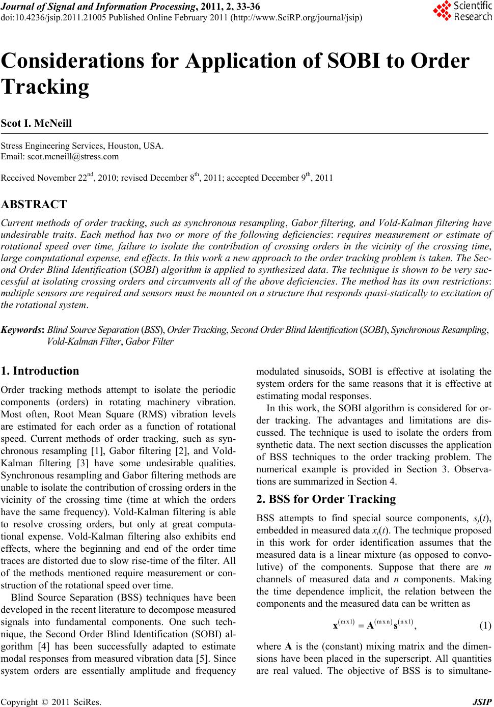Journal of Signal and Information Processing, 2011, 2, 33-36
doi:10.4236/jsip.2011.21005 Published Online February 2011 (http://www.SciRP.org/journal/jsip)
33
Considerations for Application of SOBI to Order
Tracking
Scot I. McNeill
Stress Engineering Services, Houston, USA.
Received November 22nd, 2010; revised December 8th, 2011; accepted December 9th, 2011
ABSTRACT
Current methods of order tracking, such as synchronous resampling, Gabor filtering, and Vold-Kalman filtering have
undesirable traits. Each method has two or more of the following deficiencies: requires measurement or estimate of
rotational speed over time, failure to isolate the contribution of crossing orders in the vicinity of the crossing time,
large computational expense, end effects. In this work a new approach to the order tracking problem is taken. The Sec-
ond Order Blind Identification (SOBI) algorithm is applied to synthesized data. The technique is shown to be very suc-
cessful at isolating crossing orders and circumvents all of the above deficiencies. The method has its own restrictions:
multiple sensors are required and sensors must be mounted on a structure that responds quasi-statically to excitation of
the rotational system.
Keywords: Blind Source Separation (BSS), Order Tracking, Second Order Blind Identification (SOBI), Synchronous Resampling,
Vold-Kalman Filter, Gabor Filter
1. Introduction
Order tracking methods attempt to isolate the periodic
components (orders) in rotating machinery vibration.
Most often, Root Mean Square (RMS) vibration levels
are estimated for each order as a function of rotational
speed. Current methods of order tracking, such as syn-
chronous resampling [1], Gabor filtering [2], and Vold-
Kalman filtering [3] have some undesirable qualities.
Synchronous resampling and Gabor filtering methods are
unable to isolate the contribution of crossing orders in the
vicinity of the crossing time (time at which the orders
have the same frequency). Vold-Kalman filtering is able
to resolve crossing orders, but only at great computa-
tional expense. Vold-Kalman filtering also exhibits end
effects, where the beginning and end of the order time
traces are distorted due to slow rise-time of the filter. All
of the methods mentioned require measurement or con-
struction of the rotational speed over time.
Blind Source Separation (BSS) techniques have been
developed in the recent literature to decompose measured
signals into fundamental components. One such tech-
nique, the Second Order Blind Identification (SOBI) al-
gorithm [4] has been successfully adapted to estimate
modal responses from measured vibration data [5]. Since
system orders are essentially amplitude and frequency
modulated sinusoids, SOBI is effective at isolating the
system orders for the same reasons that it is effective at
estimating modal responses.
In this work, the SOBI algorithm is considered for or-
der tracking. The advantages and limitations are dis-
cussed. The technique is used to isolate the orders from
synthetic data. The next section discusses the application
of BSS techniques to the order tracking problem. The
numerical example is provided in Section 3. Observa-
tions are summarized in Section 4.
2. BSS for Order Tracking
BSS attempts to find special source components, sj(t),
embedded in measured data xi(t). The technique proposed
in this work for order identification assumes that the
measured data is a linear mixture (as opposed to convo-
lutive) of the components. Suppose that there are m
channels of measured data and n components. Making
the time dependence implicit, the relation between the
components and the measured data can be written as
 
mx1mxnnx1 ,xAs (1)
where A is the (constant) mixing matrix and the dimen-
sions have been placed in the superscript. All quantities
are real valued. The objective of BSS is to simultane-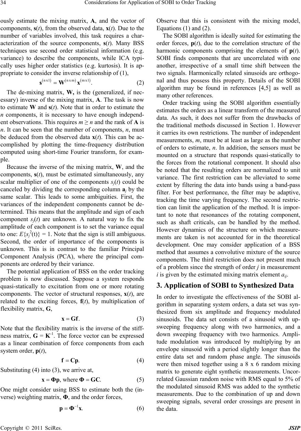

Considerations for Application of SOBI to Order Tracking 34
ously estimate the mixing matrix, A, and the vector of
components, s(t), from the observed data, x(t). Due to the
number of variables involved, this task requires a char-
acterization of the source components, s(t). Many BSS
techniques use second order statistical information (e.g.
variance) to describe the components, while ICA typi-
cally uses higher order statistics (e.g. kurtosis). It is ap-
propriate to consider the inverse relationship of (1),
 
nx1nxmmx1 .sWx (2)
The de-mixing matrix, W, is the (generalized, if nec-
essary) inverse of the mixing matrix, A. The task is now
to estimate W and s(t). Note that in order to estimate the
n components, it is necessary to have enough independ-
ent observations. This requires m ≥ n and the rank of A is
n. It can be seen that the number of components, n, must
be deduced from the observed data x(t). This can be ac-
complished by plotting the time-frequency distribution
computed using short-time Fourier transform, for exam-
ple.
Because the inverse of the mixing matrix, W, and the
components, s(t), must be estimated simultaneously, any
scalar multiplier of one of the components sj(t) could be
canceled by dividing the corresponding column aj by the
same scalar. This leads to some ambiguities. First, the
variances of the independent components cannot be de-
termined. This means that the amplitude and sign of each
component sj(t) are unknown. A natural way to fix the
amplitude of each component is to set the variance equal
to one: E{sj
2(t)} = 1. Note that the sign is still ambiguous.
Second, the order of importance of the components is
unknown. This is in contrast to the familiar Principal
Component Analysis (PCA), where the principal com-
ponents are ordered by their variance.
The potential application of BSS on the order tracking
problem is now discussed. Suppose a system responds
quasi-statically to excitation from one or more rotating
components. The vector of structural responses, x(t), are
related to the exciting forces, f(t), by multiplication of
flexibility matrix, G,
.xGf (3)
Note that the flexibility matrix is the inverse of the stiff-
ness matrix, G = K-1. The force vector can be expressed
as a linear combination of force components from each
system order, p(t),
.fCp (4)
Substituting (4) into (3), we arrive at,
,where .xΦpΦGC (5)
One might consider using BSS to estimate both the (in-
verse) weighting matrix, Φ, and the order forces,
1. 
pΦx (6)
Observe that this is consistent with the mixing model,
Equations (1) and (2).
The SOBI algorithm is ideally suited for estimating the
order forces, p(t), due to the correlation structure of the
harmonic components comprising the elements of p(t).
SOBI finds components that are uncorrelated with one
another, irrespective of a small time shift between the
two signals. Harmonically related sinusoids are orthogo-
nal and thus possess this property. Details of the SOBI
algorithm may be found in references [4,5] as well as
many other references.
Order tracking using the SOBI algorithm essentially
estimates the orders as a linear transform of the measured
data. As such, it does not suffer from the drawbacks of
the traditional methods discussed in Section 1. However
it carries its own restrictions. The number of independent
measurements, m, must be at least as large as the number
of orders to estimate, n. In addition, the sensors must be
mounted on a structure that responds quasi-statically to
the forces from the rotational component. It should also
be noted that the resulting orders are normalized to unit
variance. The first restriction can be alleviated to some
extent by filtering the data into bands using a band-pass
filter. For best performance, the filter may be adaptive,
tracking the time varying frequency. The second restric-
tion can limit the application of the method. It is impor-
tant to note that resonances of the rotating component,
such as shaft criticals, can be handled by the method.
However dynamics of the structure on which measure-
ments are taken is not accounted for in the theoretical
development. One may consider application of a BSS
method that assumes a convolutive mixture of the source
components. The third restriction does not present much
of a problem since the strength of order j in measurement
i is given by the estimated mixing matrix element aij.
3. Application of SOBI to Synthesized Data
In order to investigate the effectiveness of the SOBI al-
gorithm in separating system orders, a data set was syn-
thesized from six amplitude and frequency modulated
sinusoids. The data set consists of a sinusoid with up-
sweeping frequency along with two harmonics, and a
down sweeping frequency with two harmonics. Ampli-
tude modulation was introduced by multiplying by an
envelope sinusoid with a period slightly longer than the
entire data set and random phase angle. The sinusoids
were then mixed together using a 8 x 6 random mixing
matrix to generate eight synthetic measurements. Uncor-
related Gaussian random noise with RMS equal to 5% of
the modulated sinusoid RMS was added to the synthetic
measurements. Due to the combination of up and down
sweeping signals, several order crossings are present in
the data.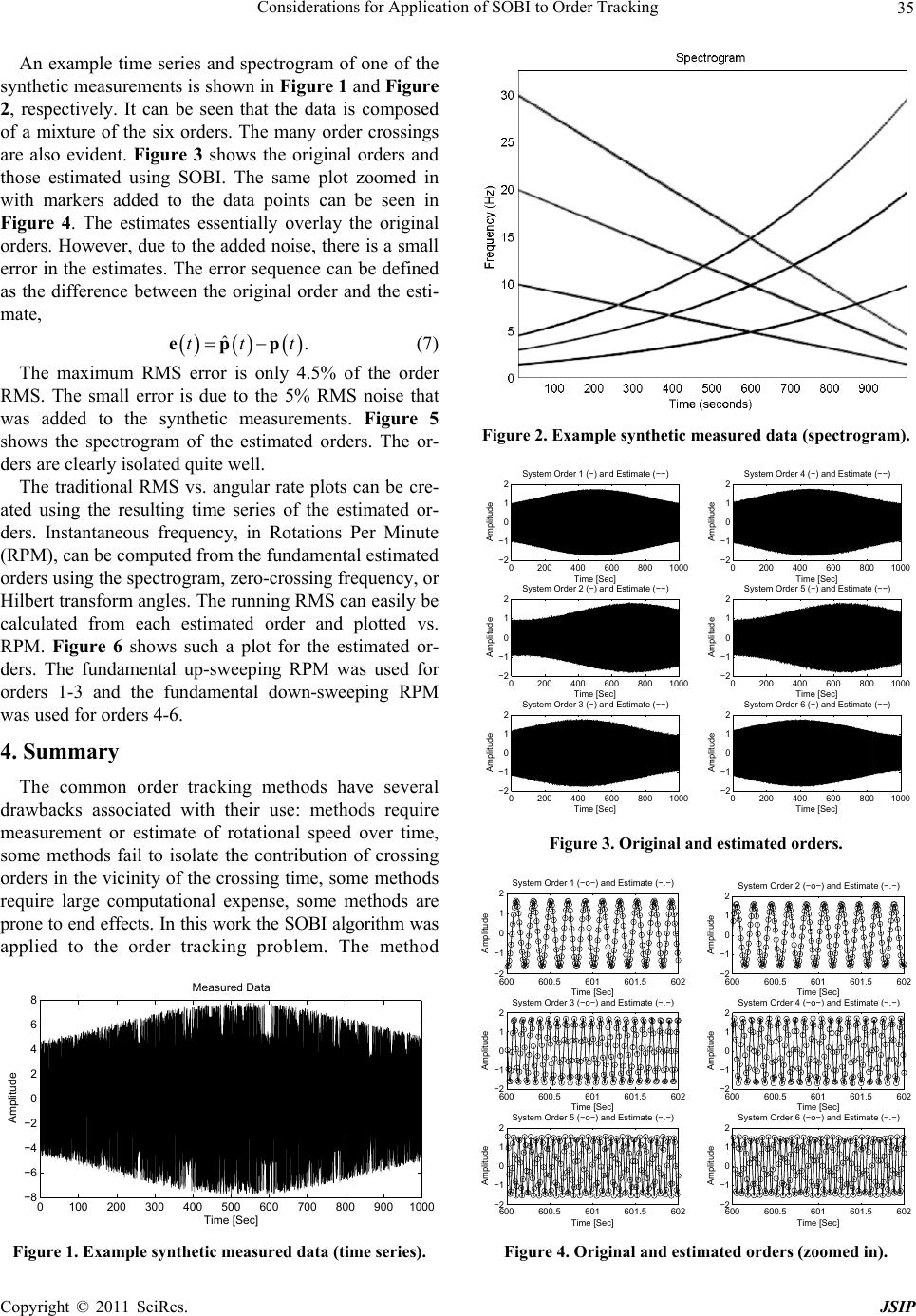

Considerations for Application of SOBI to Order Tracking 35
An example time series and spectrogram of one of the
synthetic measurements is shown in Figure 1 and Figure
2, respectively. It can be seen that the data is composed
of a mixture of the six orders. The many order crossings
are also evident. Figure 3 shows the original orders and
those estimated using SOBI. The same plot zoomed in
with markers added to the data points can be seen in
Figure 4. The estimates essentially overlay the original
orders. However, due to the added noise, there is a small
error in the estimates. The error sequence can be defined
as the difference between the original order and the esti-
mate,



ˆ.tttepp
(7)
The maximum RMS error is only 4.5% of the order
RMS. The small error is due to the 5% RMS noise that
was added to the synthetic measurements. Figure 5
shows the spectrogram of the estimated orders. The or-
ders are clearly isolated quite well.
The traditional RMS vs. angular rate plots can be cre-
ated using the resulting time series of the estimated or-
ders. Instantaneous frequency, in Rotations Per Minute
(RPM), can be computed from the fundamental estimated
orders using the spectrogram, zero-crossing frequency, or
Hilbert transform angles. The running RMS can easily be
calculated from each estimated order and plotted vs.
RPM. Figure 6 shows such a plot for the estimated or-
ders. The fundamental up-sweeping RPM was used for
orders 1-3 and the fundamental down-sweeping RPM
was used for orders 4-6.
4. Summary
The common order tracking methods have several
drawbacks associated with their use: methods require
measurement or estimate of rotational speed over time,
some methods fail to isolate the contribution of crossing
orders in the vicinity of the crossing time, some methods
require large computational expense, some methods are
prone to end effects. In this work the SOBI algorithm was
applied to the order tracking problem. The method
0100 200 300 400 500 600 700 800 900100
0
−8
−6
−4
−2
0
2
4
6
8
Time [Sec]
Amplitude
Measured Data
Figure 1. Example synthetic measured data (time series).
Figure 2. Example synthetic measured data (spectrogram).
0200 400 600 8001000
−2
−1
0
1
2
Time [Sec]
Amplitude
System Order 1 (−) and Estimate (−−)
0200 400 600 8001000
−2
−1
0
1
2
Time [Sec]
Amplitude
System Order 2 (−) and Estimate (−−)
0200 400 600 8001000
−2
−1
0
1
2
Time [Sec]
Amplitude
System Order 3 (−) and Estimate (−−)
0200 400 600 800100
0
−2
−1
0
1
2
Time [Sec]
Amplitude
System Order 4 (−) and Estimate (−−)
0200 400 600 800100
0
−2
−1
0
1
2
Time [Sec]
Amplitude
System Order 5 (−) and Estimate (−−)
0200 400 600 800100
0
−2
−1
0
1
2
Time [Sec]
Amplitude
System Order 6 (−) and Estimate (−−)
Figure 3. Original and estimated orders.
600 600.5 601 601.5 602
−2
−1
0
1
2
Time [Sec]
Amplitude
System Order 1 (−o−) and Estimate (−.−)
600 600.5 601 601.5 602
−2
−1
0
1
2
Time [Sec]
Amplitude
System Order 3 (−o−) and Estimate (−.−)
600 600.5 601 601.5 602
−2
−1
0
1
2
Time [Sec]
Amplitude
System Order 5 (−o−) and Estimate (−.−)
600 600.5 601 601.5 602
−2
−1
0
1
2
Time [Sec]
Amplitude
System Order 2 (−o−) and Estimate (−.−)
600 600.5 601 601.5 602
−2
−1
0
1
2
Time [Sec]
Amplitude
System Order 4 (−o−) and Estimate (−.−)
600 600.5 601 601.5 602
−2
−1
0
1
2
Time [Sec]
Amplitude
System Order 6 (−o−) and Estimate (−.−)
Figure 4. Original and estimated orders (zoomed in).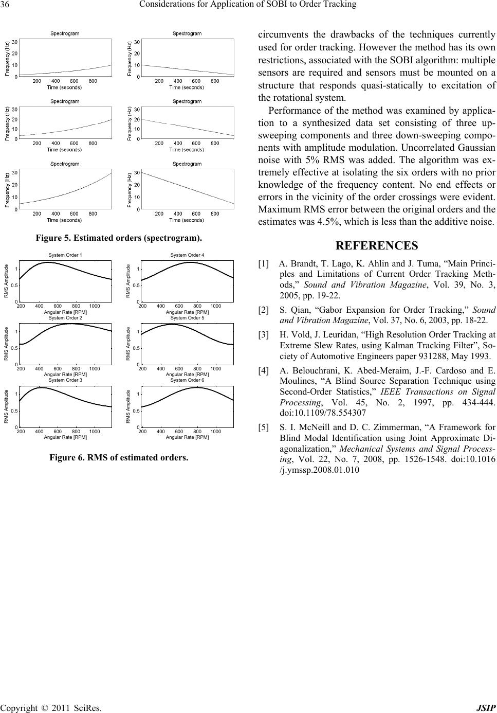

Considerations for Application of SOBI to Order Tracking 36
Figure 5. Estimated orders (spectrogram).
200 400 600 8001000
0
0.5
1
Angular Rate [RPM]
RMS Amplitude
System Order 1
200 400 600 8001000
0
0.5
1
Angular Rate [RPM]
RMS Amplitude
System Order 2
200 400 600 8001000
0
0.5
1
Angular Rate [RPM]
RMS Amplitude
System Order 3
200 400 600 8001000
0
0.5
1
Angular Rate [RPM]
RMS Amplitude
System Order 4
200 400 600 8001000
0
0.5
1
Angular Rate [RPM]
RMS Amplitude
System Order 5
200 400 600 8001000
0
0.5
1
Angular Rate [RPM]
RMS Amplitude
System Order 6
Figure 6. RMS of estimated orders.
circumvents the drawbacks of the techniques currently
used for order tracking. However the method has its own
restrictions, associated with the SOBI algorithm: multiple
sensors are required and sensors must be mounted on a
structure that responds quasi-statically to excitation of
the rotational system.
Performance of the method was examined by applica-
tion to a synthesized data set consisting of three up-
sweeping components and three down-sweeping compo-
nents with amplitude modulation. Uncorrelated Gaussian
noise with 5% RMS was added. The algorithm was ex-
tremely effective at isolating the six orders with no prior
knowledge of the frequency content. No end effects or
errors in the vicinity of the order crossings were evident.
Maximum RMS error between the original orders and the
estimates was 4.5%, which is less than the additive noise.
REFERENCES
[1] A. Brandt, T. Lago, K. Ahlin and J. Tuma, “Main Princi-
ples and Limitations of Current Order Tracking Meth-
ods,” Sound and Vibration Magazine, Vol. 39, No. 3,
2005, pp. 19-22.
[2] S. Qian, “Gabor Expansion for Order Tracking,” Sound
and Vibration Magazine, Vol. 37, No. 6, 2003, pp. 18-22.
[3] H. Vold, J. Leuridan, “High Resolution Order Tracking at
Extreme Slew Rates, using Kalman Tracking Filter”, So-
ciety of Automotive Engineers paper 931288, May 1993.
[4] A. Belouchrani, K. Abed-Meraim, J.-F. Cardoso and E.
Moulines, “A Blind Source Separation Technique using
Second-Order Statistics,” IEEE Transactions on Signal
Processing, Vol. 45, No. 2, 1997, pp. 434-444.
doi:10.1109/78.554307
[5] S. I. McNeill and D. C. Zimmerman, “A Framework for
Blind Modal Identification using Joint Approximate Di-
agonalization,” Mechanical Systems and Signal Process-
ing, Vol. 22, No. 7, 2008, pp. 1526-1548. doi:10.1016
/j.ymssp.2008.01.010