Centerline Extraction for Image Segmentation Using Gradient and Direction Vector Flow Active Contours
410
an edge indicator function
,11,
xyf xy can
be used to multiply with the magnitude of the gradient of
GVF field since the edge function is very small when the
pixel at (x, y) is on the strong edge and has a value of 1 in
other places. In summary, centerlines can be extracted by
first calculating the product of the magnitude of the gra-
dient of GVF field and the edge indicator function,
,,,k xygxyxyv, (11)
then normalizing it to [0, 1],
,min
,
max min
q
kxy k
kxy kk
,
(12)
and finally comparing with a threshold
1,
,0,
if kx yT
sxy
else
,
,
(13)
where T is a pre-set threshold between 0 and 1. In Equa-
tion (12), q is the field strength taking a value between 0
and 1, which can be used to control the centerline strength.
Morphological operations such as opening can be applied
to process the threshold result
,
xy B (14)
where B is a structuring element, and “o” denotes a
morphological opening operation. If necessary, thinning
or skeleton algorithm can be further used to make the
extracted lines thinner. Once the centerlines are extracted,
the G & DVF users will know where the best place is to
draw the directional lines and generate the DVF field.
That is, the users can just simply follow the detected cen-
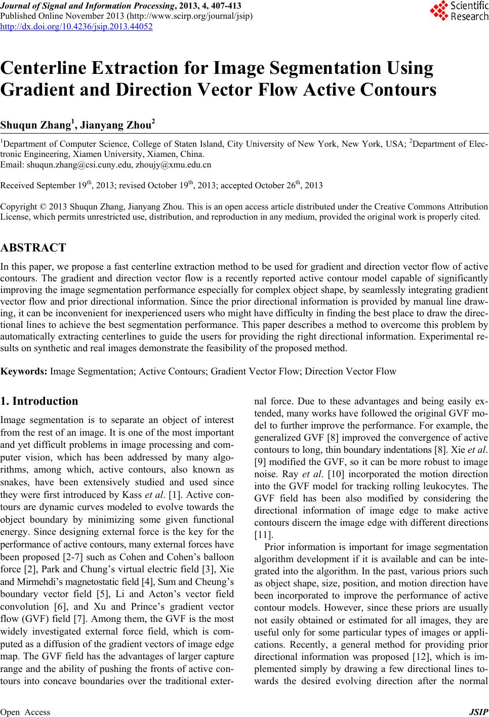
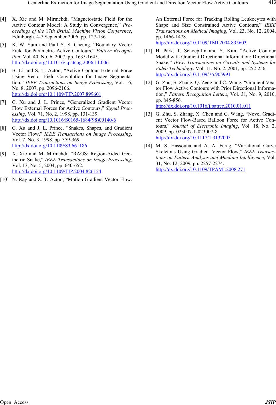
terlines to draw the directional lines. As an example, Fig-
ure 1(d) shows the centerline extraction result from Fig-
ure 1(a) using the proposed method described above,
where lines outside the object support has been removed.
The required directional lines (shown in red color) for the
G & DVF can be easily obtained based on Figure 1(d),
which are similar to the lines shown in Figure 1(a).
It is noted that the proposed method has very low com-
putational complexity since it simply utilizes the already
computed GVF for centerline extraction and there is no
much extra calculation needed.
3. Experimental Results
To demonstrate the feasibility of the proposed method,
we present experiments tested on both synthetic and real
images. The image size is 120 × 120 pixe ls for the tested
synthetic image, while is 240 × 240 pixels for the tested
real image. In the experiments, the edge maps for com-
puting the force fields are normalized to the range [0, 1].
The parameters α = 0.8, β = 0.0, and µ = 0.2 were chosen
for both the G & DVF and the GVF, and η = 1.5 for the
G & DVF. The field strength q = 1 is used. The GVF and
G & DVF active contours use the same circle-shaped ini-
tializations in each of our experiments, which are not plac-
ed in the neighbor h ood of t he d e s i r ed obje c t b oundar y.
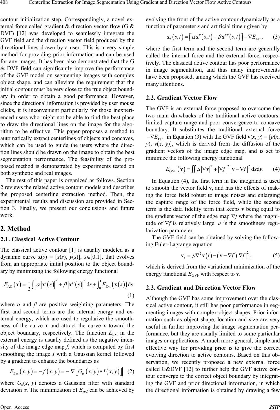
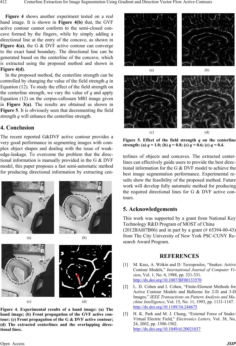
Figure 2 shows an experiment tested on a synthetic
“S” shape image. The original image is shown in Figure
2(a). The two semi-closed concaves formed in the “S”
shape are difficult for the original GVF field to handle
and the contour is usually stuck at the entries. This can
be seen from Figure 2(b) that shows the segmentation
result using the original GVF model. The failure of seg-
mentation using the original GVF is because there are
some GVF field vectors pointing outward at the entry of
the semi-closed concave as shown in Figure 2(c), which
prevents the front of the GVF active contour moving into
the semi-closed concave boundary. For better segmenting
the “S” sh ape image, we can use the G & DVF and dr aw
two directional lines at the entries of the two semi-closed
concaves as shown in Figure 2(e) to force the field vec-
tor to point inward. The field vector change from out-
ward to inward is demonstrated in Figure 2(d), which
shows the G & DVF field vectors at the entry of the
semi-closed concave. The changing of field vector direc-
tion helps the front of the G & DVF active contour exact-
ly propagate into the semi-closed concave as shown Fig-
ure 2(f). The two drawn lines shown in Figure 2(e) ac-
tually can be extracted using the proposed method. Fig-
ure 2(g) shows the detection result of the centerlines us-
ing the proposed method. Given Figure 2(g), the G &
DVF users will know where exactly to draw the direction
lines, simply following the centerlines as shown in Fig-
ure 2(h). Alternatively we can also automatically pro-
duce a line by finding the two end points of a detected
area.
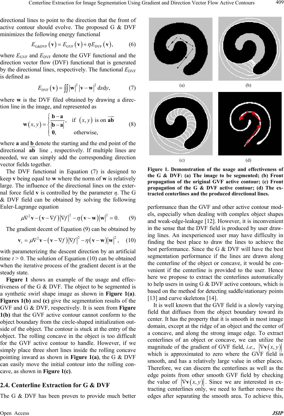
Another experiment was performed on a real corpus-
callosum MRI image as shown on Figure 3(a). The ac-
tive contour is initialized at one end of the corpus-callo-
sum. We expect that the front of the active contour mov es
into a hooked con cave for exactly co nforming to th e cor-
pus-callosum boundary. The segmentation result using
the original GVF model is given in Figure 3(b), where
the GVF field obviously cannot drive the front of the
GVF active contour to move into the hooked concave,
and the front of the GVF active contour stops moving at
the beginning of the hooked concave. With the G & DVF
active contour, simply drawing three directional lines on
the image will assist the curve evolution, as shown in
Figure 3(c). The corresponding segmentation result by
the G & DVF is shown in Figure 3(d). It successfully
drives the front of the active contour to the correct object
boundary from the circle-shaped initialization. The ob-
tained different results for these two models can be ex-
plained from their vector fields as shown in Figures 3(e)
and (f), where the GVF field vectors point to many dif-
Open Access JSIP