Journal of Applied Mathematics and Physics, 2013, 1, 63-67
http://dx.doi.org/10.4236/jamp.2013.14012 Published Online October 2013 (http://www.scirp.org/journal/jamp)
Kriging of Airborne Gravity Dat a in the
Coastal Ar e as of th e Gulf of Mexi co
Hongzhi Song, Alexey L. Sadovski, Gary Jeffress
Conrad Blucher Institute, Texas A&M University-Corpus Christi, Corpus Christi, USA
Received July 2013
ABSTRACT
This paper deals with the application of kriging technique to find the continuous map of gravity on the geoid in the
coastal areas and to evaluate its precision.
Keywords: Gravity; Kriging; Geoid; Map; Statistics
1. Introduction
By using satellites, scientists discovered the long wave
(large scale) geoid for the Earth (Seeber, 2003; Drink-
water et al., 2003) [1], but its resolution is not sufficient
for orthometric height determination from GPS when it
comes to the relatively small scale and/or local events
such as flooding. This was the case after flooding created
by storm surges fr om hurri can es Katri na, R ita (2 005), a nd
Ike (2008) in the coastal areas of the Gulf of Mexico. So,
there is a need to develop method(s) and model(s) of the
geoid determination at the local level, based on local
observations of gravity, and complemented by observa-
tions of gravity from the air and space.
In principle, there is a need for gravity g at every point
of the Earth’s surface. Gravity is continuously changing,
and it reflects the results of Earth’s phenomena, such as
tropic storm, hurricane, earthquake, early tides, variation
in the atmosphere density, etc. Gravity also alters when
only a small change happened in the constructions and
the density of materials beneath the constructions. But
having gravity data provided everywhere on the Earth is
totally impossible in reality. To predict values of a ran-
dom unsampled area from a set of observations is needed.
It is well known that the kriging method is not the best
approach to predict free-air gravity anomalies, but in this
paper, we assume that the kriging method is a better ap-
proach than other methods for prediction of gravity based
on the airborne data provided by National Geodetic Sur-
vey (NGS). The result we still have a confidence in the
kriging method is that the kriging method can estimate
the prediction error to assess the quality of a prediction.
This function makes the kriging method with a big dif-
ference from other methods.
2. Data
Data used in this chapter is airborne gravity data of the
Gravity for the Redefinition of the American Vertical
Datum (GRAV-D) project which was released by NGS
[2]. Table 1 lists the nominal block characteristics, and
details can be founded in GRAV-D General Airborne
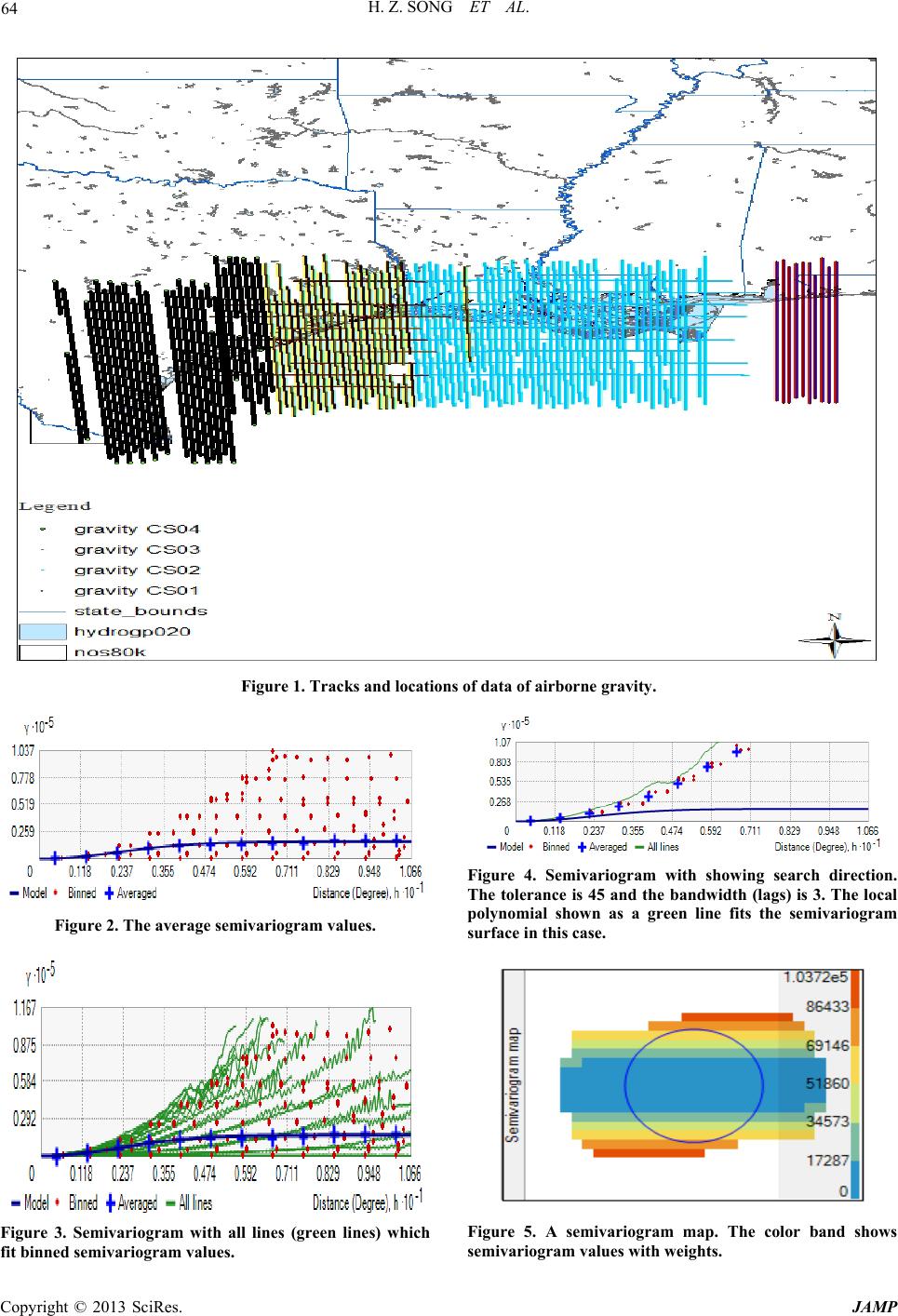
Gravity Data User Manual. Four blocks (Block CS01,
CS02, CS03 and CS04) data (Figure 1) were chosen to
be interpolated.
The total sample size (four blocks together) is 389578,
and the gravity values range between 975480 mGal and
977490 mGal. Keep in mind, the standard gravity is
980665 mGal. The airborne gravity data was fixed by
using free-air reduction and by the international gravity
formula [3].
3. Kriging of Gravity on the Geoid
The kriging method here was conducted by using Arc-
GIS 10.1—Spatial Analyst and Geostatistical Analyst.
There are six different types of kriging in Geostatistical
Analyst tools. The most common types are ordinary
kriging and universal kriging, which were chosen to be
used in this study. The simple kriging method is also
Table 1. Nominal data characteristics.
Characteristic Nominal Value
Altitude 20, 000 ft (~ 6.3 km)
Ground speed250 knots (250 nautical miles/hr)
Along-track gravimeter sampling1 sample per second = 128.6 m (at nominal ground speed)
Data Line Spacing10 km
Data Line length400 km
Cross Line Spacing40-80 km
Cross Line Length500 km
Data Minimum Resolution20 km

H. Z. SONG ET AL.
64
Figure 1. Tracks and locations of data of airborne gravity.
Figure 2. The average semivariogram values.
Figure 3. Semivariogram with all lines (green lines) which
fit binned semivariogram values.
Figure 4. Semivariogram with showing search direction.
The tolerance is 45 and the bandwidth (lags) is 3. The local
polynomial shown as a green line fits the semivariogram
surface in this case.
Figure 5. A semivariogram map. The color band shows
semivariogram values with weights.

H. Z. SONG ET AL.
65
quite common, but it requires that the data should have
normal distribution. Thus, the simple kriging method was
not applied in this study. There are three major compo-
nents—the spatial autocorrelation component (known as
semivariogram), a trend, and a random error term. These
three components are the key to lead to different types of
the kriging methods. The simple equation represents the
kriging method is:
1
n
s ii
i
z zw
=
=
∑
, where zs is the esti-
mated value for an unsampled location s; zi is the known
value at the control point i; wi represents the weight ap-
plied to sample values assoc iated with the control poin t i;
n is the number of sample points used in the estimation.
The averaged semivariogram values on the y-axis (in
mgal2), and distance (or lag) on the x-axis (in degree).
Binned values are shown as red dots, which are sorted
the relative values between points based on their dis-
tances and directions and computed a value by square of
the difference between the original values of points; Av-
erage values are shown as blue crosses, which are gener-
ated by binning semivariogram points; The model is
shown as blue curve, which is fitted to average values.
Model: 28.118 * Nugget + 16437 * Stable (5.53,2);
Model: 28.118 * Nugget + 16437 * Gaussian (5.53).
The predicted, error, standard error, and normal QQ
plot graphs are plotted respectively in Figures 6(a)-(d).
The predicted graph shows how well the known sample
value was predicted compared to its actual value. The
regressi on funct i on in Figure 6(a) is
(x)0.9999x 125.1751f= +
. By visually analyzed the
graph, the regression function is closely aligned with the
reference line. Therefore, it is well predicted.
The error graph shows the difference between known
values and predictions for these values. The error equa-
tion in Figure 6(b) is
10.00001 127.1751yx= +
. The
standardized error graph shows the error divided by the
estimated kriging errors. The standardized error equation
in Figure 6(c) is
10.00002 22.9974yx= +
. The normal
QQ plot of the s tandardiz ed error Figure 6(d) shows how
closely the difference between the errors of predicted and
actual values align with the standard normal distribution
(the reference line). Figures 7 and 8 demonstrate the
prediction and standard error map by using the ordinary
kriging with stable and Gaussian techniques.
Trend analysis was presented in Figure 9. T here is no
trend exists because the curve through the projected
points is flat (as shown by the light blue line in the Fig-
ure 9). A slight downward curve as shown by the red
line in Figure 9 is through the projected points on ZY
plane, which suggests that it may have a trend exist in
gravity on the geoid data. Therefore, de-trend is con-
ducted before the universal kriging process in order to
prevent biased the analysis. Because the curve shown on
ZY plane is not obvious, the de-trend approach is chosen
(a) ( b)
(c) (d)
Figure 6. Cross validation of the ordinary kriging.

H. Z. SONG ET AL.
66
Figure 7. The ordinary stable and Gau s sian kriging predictions map.
Figure 8. The or dinary stable and Gau ss i an kriging prediction standar d error map.
to remove the trend order as constant. The process was
conducted in ArcGIS 10.1 by using Geostatistical Ana-
lyst. Results of the universal kriging with either the sta-
ble technique or the Gaussian technique were shown as
exact the same as results of the ordinary kriging.
Legend: Grid (XYZ): Number of Grid Lines 11 × 11 ×
6; Projected Data: YZ plane (Dark Blue), ZY plane
(Yellow), XY plane (Peony Pink); Trend on Projections:
YZ plane (Light Blue), XZ plane (Red); Axes (Black).
A better interpolation method should have a smaller
RMS. Due to no difference between the ordinary kriging
and universal kriging in this case; statistical results were

H. Z. SONG ET AL.
67
Table 2. Statistics.
RMS Standardized 0.1084
Mean Standardized 0.0007
Average Standard Erro r (ASE) 5.5060
Root Mena Square (RMS) 0.5918
Difference between
RMS and ASE 4.9142
Difference in Percentage 89.25%
Figure 9. Trend analysis of gravity on the geoid.
Figure 10. The ordinary kriging predictions map of gravity on the geoid along Gulf of Mexico coast.
the same which listed in Table 2. The prediction error
mean is 0.0038 mGal. As 1 meter increased in altitude,
the gravity is decreased by 0.3086 mGal. With simple
conversion, the accuracy of prediction is approximately
0.0123 meters. Namely, it is around 1.23 cm, which was
expected.
REFERENCES
[1] M. R. Drinkwater, R. Floberghagen, R. Haagmans, D.
Muzi and A. Popescu, “VII: CLOSING SESSION:
GOCE: ESA’s First Earth Explorer Core Mission,” Space
Science Reviews, Vol. 108, No. 1-2, 2003, pp. 419-432.
http://dx.doi.org/10.1023/A:1026104216284
[2] GRAV-D Science Team, “GRAV-D General Airborne
Gravity Data User Manual,” Theresa M. Diehl, Ed., Ver-
sion 1, 2011.
http://www.ngs.noaa.gov/GRAVD/data_cs01.shtml
[3] X. Li and H. J. Götze, “Tutorial Ellipsoid, Geoid, Gravity,
Geodesy, and Geophysics,” Geophysics, Vol. 66, No. 6,
2001, pp. 1660-1668.
http://dx.doi.org/10.1190/1.1487109
[4] B. Hofmann-Wellenhof and H. Moritz, “Physical Geode-
sy,” 2nd Edition, Springer Wien, New York, 2006.