Journal of Applied Mathematics and Physics, 2013, 1, 6-11
http://dx.doi.org/10.4236/jamp.2013.14002 Published Online October 2013 (http://www.scirp.org/journal/jamp)
Parall el Simul at ion of 3D Wave Propagati on by Doma in
Decomposition
Galina Reshetova1, Vladimir Tcheverda2, Dmitry Vishnevsky2
1The Institute of Computational Mathematics and Mathematical Geophysics, Siberian Branch of the RAS, Russia
2The Institute of Petroleum Geology and Geophysics, Siberian Branch of the RAS, Russia
Received July 2013
ABSTRACT
In order to perform large scale numerical simulation of wave propagation in 3D heterogeneous multiscale viscoelastic
media, Finite Difference technique and its parallel implementation based on domain decomposition is used. A couple of
typical statements of borehole geophysics are dealt with—sonic log and cross well measurements. Both of them are
essentially multiscales, which claims to take into account heterogeneities of very different sizes in order to provide re-
liable results of simulations . Locally refined spatial grids help us to avoid the use of redundantly tiny grid cells in a tar-
get area, but cause some troubles with uniform load of Processor Units involved in computations. We present r esults of
scalability tests together with results of numerical simulations for both statements performed for some realistic models.
Keywords: Seismic Wave propagation; Sonic Log; Numerical Simulation; Domain Decomposition
1. Introduction
The most effective way to improve resolving ability of
any wave ima ges is to increase dominant frequency of a
sounding pulse. But Earth media attenuate and disperse
propagating waves. Both these effects are often quanti-
fied by the Quality Factor Q. This factor describes rela-
tive dissipation of seismic energy per unit volume per
unit cycle. If attenua tion is not too strong, Quality Factor
can be treated as a number of wavelengths a wave can
propagate through a medium before its amplitude was
decreased in
π
e
time s.
Both fields and laboratory experiments prove that this
parameter can be treated as independent on time fre-
quency for rather wide frequency range [5]. Therefore
the higher is the dominant frequency of a source pulse,
the shorter is the distance with reliable level of sig-
nal-to-noise ratio. So, in order to get an image with high
resolution it is necessary to place acquisition system as
close to the target object as possible. The only way to do
this is to place sources and/or receivers within boreholes
drilled in the vicinity of the targ et object. I n its own turn
presence of a well filled with a drilling mud brings es-
sential peculiarities to wave fields and should be taken
into account in model description. In its own turn, this
claims use of locally refined grids in order to catch hete-
rogeneities of the smallest scale only.
The paper deals with numerical simulation of waves
propagation within viscoelastic media for the following
borehole ba s ed geophysical methods:
a) Sonic Log—sources and receivers are within the
same borehole and the main task is monitoring of casing
pipe integrity and recovery of near well-bore vicinity.
Multiscale nature of the problem becomes apparent in the
presence of heterogeneities of at least two different
scales-distance source/receiver and borehole radius. If
one deals with a cased borehole there is third scale-
structure of the casing. Fourth scale can be introduced by
a medium;
b) Cros s-well Tomography—sources and receivers
are placed within adjacent boreholes encircling a target
object. This problem possesses two extremely different
scales-borehole diameter and distance between sources
and receivers.
2. Viscoelastic Media
Any process of wave propagation within linear elastic
medium is governed by t w o groups of eq ua tions:
1) Motion equations (Newton’s law);
2) State equation that connects stress and strain tensors
(Hook’s law).
In reality rocks possess intrinsic attenuation produced
by their “memo ry”: stress state at some instant t is de-
termined by the “history” of strains. We will suppose that
all processes are causal, that is the current state of the
medium does not depend on the future by no means. So,
in the most general form the Hook’s law for these mate-

G. RESHETOVA ET AL.
7
rials can be written down in the following way:
( )( )
0
(,) (,0)(,)
,
,
ijijkl kl
tkl
ijkl
xtG xxt
xt
Gx d
σε
ετ
ττ
τ
= +
∂−
+∂
∫
For isotropic viscoelastic materials relaxation tensor
simplifies to the follo wing one:
Λ(,) 2(,)
ijklij klikjl
GxtM xt δδ δδ = +
Numerical resolution of integro-differential equations
(1) is very troublesome. The most convenient way is to
represent state equation in a differential form on a base
of mechanical analog of a viscoelastic material like a set
of rings and plungers known as Generalized Linear
Standard Solid (see [2]). Moreover, real data, both field
and laboratory, proved that (see [5-7]): A correct model-
ing scheme should yield a constant Quality Factor Q and
the corre sponding di spersion r e lation.
The common way to implement these properties of
real media in mathematical model is again just men-
tioned Generalized Standard Linear Solid (GSLS). For
this model the Hook’s law is written down as:
1
;
L
j
j
σσ
=
=
∑
i
iiR i
M
tt
σε
σε
σ τετ
∂∂

+=+

∂∂

and introduces Quality Factor as:
2
22 1
22
1
1
11
() ()
1
Lll
ll
Lll
ll
L
Q
σε
σ
εσ
σ
ωτ τ
ωτ
ωωτ τ
ωτ
=
=
+
−+ +
=−
+
∑
∑
The problem is how to choose a set of parameters
,
ii σε
ττ
providing desired behavior of Quality Factor
over a predefined interval of time frequencies.
We resolve it on the base of Least Squares techniques:
2
1
1 12
(,)|( )|minJQ Qd
ω
σε ω
ττω ω
−−
= −→
∫
In order to find desired sets of relaxation times we ap-
plied
τ
-method proposed in [1] and modified recently in
[3]. Its main advantage is essential reduction of a number
of relaxation times-for realistic values of Quality Factor
(
10Q>
) one can manage with single value of
ε
τ
(and
keep it the same through the target area!) and a couple o f
σ
τ
. Application of
τ
-method for GSLS gives the fol-
lowing representation of Hook’s law:
10
(, )(1)(, )
1(,)
l
R
t
t
L
Rll
tx MLtx
Me xd
σ
τ
τ
σ
σ τε
τετ τ
τ
−
−
=
=+−
−∑∫
Let us diffe rentiate this relation with respect to time
t
:
() ( )
( )( )
0
1
,
1
11
,,
l
RR
t
Lt
lll
tx
ML M
tt
txex d
σ
τ
τ
σσ
ε
σττ
εετ τ
ττ
−
−
=
∂
∂=+−
∂∂

×−



∑∫
and introduce l-th memory variable
( )()
0
1
(, ),,]
l
t
t
lR
ll
rtxM txex
σ
τ
τ
σσ
τε ετ
ττ
−
−
=−− 
∫
(2)
Straightforward differentiation of (2) provides the fol-
lowing equation for this variable:
(, )
ll
R
ll
r rtx
v
M
tx
σσ
τ
ττ
∂∂
=−−
∂∂
and we come to the following system of first-order PDE
for viscoe l a s t ic wave pr o pa ga tion:
v
tx
σ ∂∂
=
∂∂

1
(1 )
L
Rl
l
v
ML r
tx
στ
=
∂∂
=++
∂∂
∑
1
l
Rl
l
rv
Mr
tx
σ
τ
∂∂

=−+

∂∂

As one can see, implementation of GSLS claims extra
independent “memor y” variables per relaxation mechan-
ism per stress component. In particular, for 3D models 
mechanisms claim
6L
new variables besides three dis-
placements and six stresses. This leads to significant in-
crease of memory demands for simulation of waves’
propagation.
3. Parallel Implementation
Parallel Implementation is based on repr esentation of the
area of computations as superposition of disjoints sub-
domains touching one another along some contact sur-
face. Each of them is assigned to specific Processor Unit
(PU). Waves traveling in the model pass through differ-
ent subdomains, which require communication between
neighboring processors. Es sentially different geometry o f
the target area used in Sonic Log and Cross-hole Tomo-
graphy claims necessity of different approaches to Do-
main Decomposition (DD) as well. Let us consider both
of them.
3.1. Sonic Log
Target area for this statement is a circular cylinder
around the well with essential prevalence of its length in
comparison with width-typical length is about 10/12 me-
ters, while radius of this target area is no more th an 1/15

G. RESHETOVA ET AL.
8
meters. Taking this into account we slice the total 3D
model into a number of disc-like subdomains Ω. Finite
difference scheme assumes communication between
neighboring processors requiring them to exchange func-
tion values on the interfaces between elementary discs.
It should be noted that DD on the base of this rather
simple geometry easily provides possibility to guarantee
uniform load of Processor Units involved in computa-
tions. Another advantage of the chosen DD is in ex-
tremely small portions of data PU should interchange at
each time step and, so, extremely small waiting period
before computation on the next time step would be done.
The MPI (Message Passing Interface) library is applied
for arranging the above-mentioned send/receive proce-
dures and special efforts are paid in order to minimize
idle time of Processor Units due to the data exchange. In
order to provide this we start computations for each sub-
domain from its interior widening them towards inter-
faces and use non-blocking functions Isend and Ireceive
in order to arrange data exchange between neighboring
PU.
Special attention was paid to analysis of effectiveness
and scalability of this approach. This analysis was per-
formed by the series of numerical experiments performed
on the cluster HKC-160 (Siberian Supercomputer Center,
Novosibirsk) made of 80 computation modules (hp Inte-
grity rx1620 with two PU Intel Itanium 2, each of 1.6
Ghz, 3 Mb cache, 4 Gb RAM) connected via 24-port
commutator InfiniBand (10 Gbot, Cluster Interconnect).
Peak performance of the cluster is about 1 Tflop/s.
In order to estimate effectiveness of parallelization , fixed
computational area was decomposed on different quanti-
ty of subdomains, so simulation was performed for the
same target area, but with increasing number  of PU.
For each effectivenes s is found as
4* (4)
() * ()
time
eff nntime n =
(3)
where
()timen
is computer time expended by  PU
for simulation. We start with
4n=
in order to provide
from the very beginning the same amount of data ex-
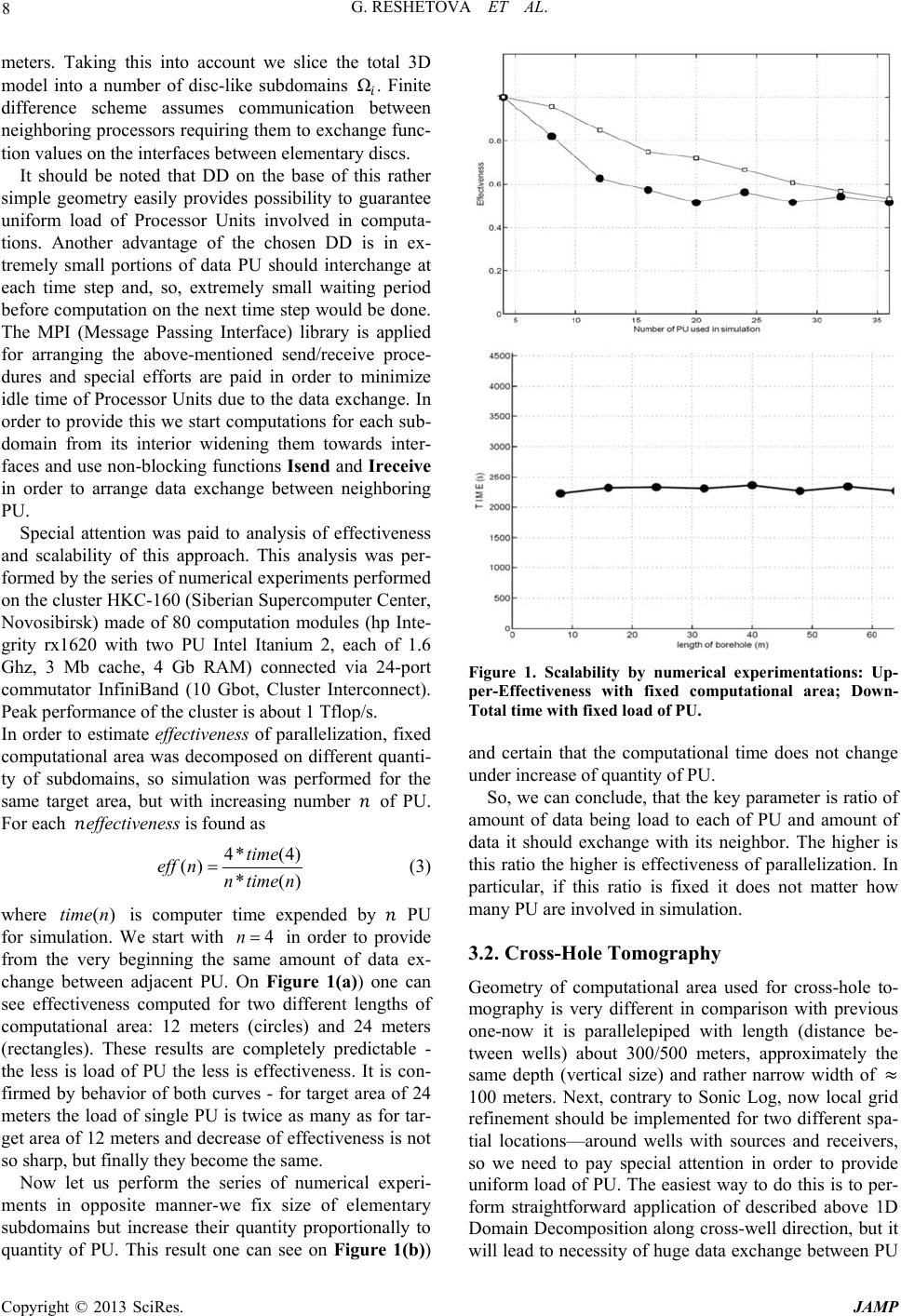
change between adjacent PU. On Figure 1(a)) one can
see effectiveness computed for two different lengths of
computational area: 12 meters (circles) and 24 meters
(rectangles). These results are completely predictable -
the less is load of PU the less is effectiveness. It is con-
firmed by behavior of both curves - for target area of 24
meters the load of single PU is twice as many as for tar-
get area of 12 meters and decrease of effectiveness is not
so sharp, but finally they become the same.
Now let us perform the series of numerical experi-
ments in opposite manner-we fix size of elementary
subdomains but increase their quantity proportionally to
quantity of PU. This result one can see on Figure 1(b))
Figure 1. Scalability by numerical experimentations: Up-
per-Effectiveness with fixed computational area; Down-
Total time with fixed load of PU.
and certain that the computational time does not change
under increase of quantity of PU.
So, we can conclude, that the key parameter is ratio of
amount of data being load to each of PU and amount of
data it should exchange with its neighbor. The higher is
this ratio the higher is effectiveness of parallelization. In
particular, if this ratio is fixed it does not matter how
many PU are involved in simulation.
3.2. Cross-Hole Tomography
Geometry of computational area used for cross-hole to-
mography is very different in comparison with previous
one-now it is parallelepiped with length (distance be-
tween wells) about 300/500 meters, approximately the
same depth (vertical size) and rather narrow width of ≈
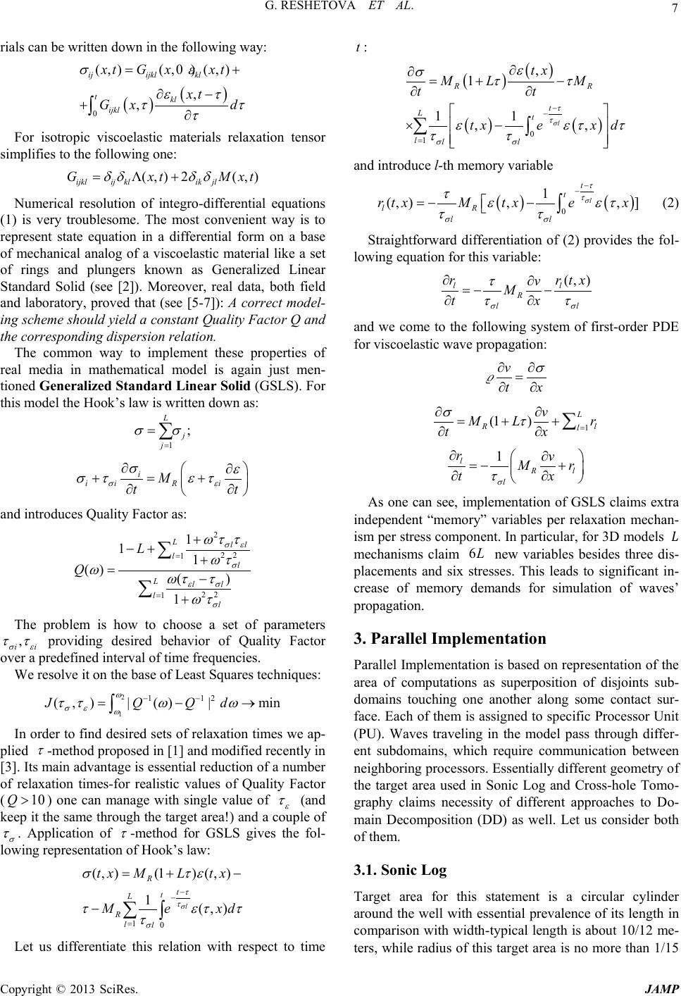
100 meters. Next, contrary to Sonic Log, now local grid
refinement should be implemented for two different spa-
tial locations—around wells with sources and receivers,
so we need to pay special attention in order to provide
uniform load of PU. The easiest way to do this is to per-
form straightforward application of described above 1D
Domain Decomposition along cross-well direction, but it
will lead to necessity of huge data exchange between PU

G. RESHETOVA ET AL.
9
produced by wide contact surface between adjacent sub-
domains which leads to essential loss of parallelization
effectiveness. In order to minimize amount of data ex-
changed between PU we need to reduce surface area of
subdomains under fixed number of grid points per each
PU—that is to choose them as close to cubes as possible.
Under this approach each PU interchange data with 3/6
neighbors.
4. Numerical Experiments
To conclude the paper let us briefly consider simulation
results for a couple of realistic models performed on the
previously descri bed cluster HKC-160.
Sonic Log
The series of numerical experiments have been imple-
mented for a range of source frequencies, positions and
models of surrounding elastic media. For illustration let
us consider the model with well completion and vertical
crack presented on the Figures 2 and 3 and possesses the
following structure:
1) Vertical borehole with radius 0.1 m filled with a mud
with
p
V
=1500 m/s,
1000= 
kg/m3, Quality Fac-
tor
65Q=
;
2) Steel tube encircling borehole; its width is equal to
0.01 m, wave propagation velocities
5600
p
V=
m/s,
3270
s
V=
m/s, =7830 kg/m3, Quality Factor
100Q=
;
3) The casing around steel tube; its width is equal to
0.04 m, its elastic parameters are the following:
p
V
= 4200 m/s,
s
V
= 2425 m/s,

= 2400 kg/m3,
Quality Factor
80Q=
;
4) Background-homogeneous viscoelastic layer with
wave propagation velocities
p
V
= 4989 m/s,
s
V
=
2605 m/s,

= 2400 kg/m3, Quality Factor
100Q=
;
5) Background-homogeneous viscoelastic layer with
wave propagation velocities
p
V
= 3208 m/s,
s
V
=
1604 m/s,

= 2400 kg/m3, Quality Factor
60Q=
;
Figure 2. Radial and azimuthal grid refinement around wel l
completion.
Figure 3. Upper—Vertical cross-section of the model; Mid-
dle—Horizontal cross-section of the model; Down—Zoomed
version of Middle figure.
6) Background-homogeneous viscoelastic layer with
wave propagation velocities
p
V
= 2650 m/s,
s
V
=
1219 m/s,

= 2400 kg/m3, Quality Factor
15Q=
;
7) Vertical crack started at r = 0.18 m and finished at r =
0.55 m, with 0.02 m in width ((see images b) and c))
filled with the same mud as within the borehole.
On the Figure 4 one can see snapshots stress rr σ

G. RESHETOVA ET AL.
10
Figure 4. Snapshots for
rr
σ
propagating through the plane
(, )0π φ =
. Left column-the model without crack; Right col-
umn-difference between the calculations for the model with and without vertical crack.
during its propagation within borehole and adjacent rocks
with and without of vertical crack. There is a series of
snapshots for components through the plane
(0,π) ϕ =
for axial source position with dominant frequency of 10
kHz located in
0.5z=
m. Two vertical red lines are
projections of interface between borehole and its com-
pletion with surrounding rocks, black horizontal lines
indicate interfaces of the layers and blue lines follow the
crack. The left column figures illustrate wave propaga-
tion for the model without of crack, while the right col-
umn figures represent the propagation of difference be-
tween the wave field with and without of crack.
5. Conclusion
The current version of developed software for simulation
of wave propagation in 3D heterogeneous viscoelastic
multiscale media opens possibility of careful study of a
rather wide range of realistic problems connected with
borehole-based geophysics. Of course, this version is not
perfect and should be further developed in different di-
rections. In particular, one of the most challenging prob-
lems is to perform full scale simulation for media with
extremely different scales, especially with microstructure
like caverns, pores and so on. In order to do that with
reasonable computer cost, one should be able to refine

G. RESHETOVA ET AL.
11
locally not spatial grid cells only, but time step used for
computations as well. Another important axis of devel-
opment is connected with necessity to provide an oppor-
tunity to perform simulation for more realistic mechani-
cal models and above all media with anisotropy induced
by fine layering, clusters of microcracks and stresses
around a well.
6. Acknowledgements
This work was supported by the Russian Foundation for
Basic Research (projects no. 11 -05-00947, 13-05-00076
and 13-05-12051).
REFERENCES
[1] J. O. Blanch, J. O. A. Robertsson and W. W. Symes ,
“Modeling of a Constant Q: Methodology and Algorithm
for an Efficient and Optimally Inexpensive Viscoelastic
Technique,” Geophysics, Vol. 60, No. 1, 2005, pp. 176-
184.
[2] R. M. Christensen, “Theory of Viscoelasticity—An In-
troduction,” Academic Press, Waltham, 1982.
[3] S. Hestholm, et al., “Quick and Accurate Q Parameteriza-
tion in Viscoelastic Wave Modeling,” Geophysics, Vol.
71, No. 5, 2006, pp. T147-T150.
[4] V. I. Kost in, D. V. Pissarenko, G. V. Reshetova and V. A.
Tcheverda, “Numerical Simulation of 3D Acoustic Log-
ging,” Lecture Notes in Computer Sciences, Vol. 4699,
2007, pp. 1045-1054.
http://dx.doi.org/10.1007/978-3-540-75755-9_122
[5] F. J. McDonal, F. A. Angona, R. L. Mills, R. L. Sengbush,
R. G. van Nostra nd and J. E. White, “Attenuation of Shear
and Compressional Waves in Pierre Shale,” Geophysics,
Vol. 23, No. 3, 1958, pp. 421-439.
http://dx.doi.org/10.1190/1.1438489
[6] S. A. Siddiqui, “Dispersion Analysis of Seismic Data,”
M.S. Thesis, University of Tulsa, Tulsa, 1971.
[7] P.C. Wuenschel, “Dispersive Body Waves—An Experi-
mental Study,” Geophysics, Vol. 30, No. 4, 1965, pp.
539-551. http://dx.doi.org/10.1190/1.1439620