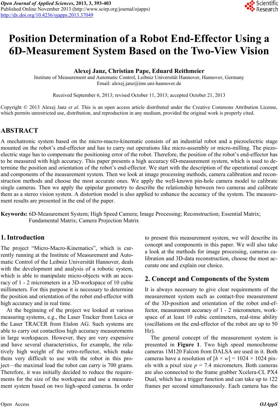
 Open Journal of Applied Sciences, 2013, 3, 393-403 Published Online November 2013 (http://www.scirp.org/journal/ojapps) http://dx.doi.org/10.4236/ojapps.2013.37049 Open Access OJAppS Position Determination of a Robot End-Effector Using a 6D-Measurement System Based on the Two-View Vision Alexej Janz, Christian Pape, Eduard Reithmeier Institute of Measurement and Automatic Control, Leibniz Universität Hannover, Hannover, Germany Email: alexej.janz@imr.uni-hannover.de Received September 6, 2013; revised October 11, 2013; accepted October 21, 2013 Copyright © 2013 Alexej Janz et al. This is an open access article distributed under the Creative Commons Attribution License, which permits unrestricted use, distribution, and reproduction in any medium, provided the original work is properly cited. ABSTRACT A mechatronic system based on the micro-macro-kinematic consists of an industrial robot and a piezoelectric stage mounted on the robot’s end-effector and has to carry out operations like micro-assembly or micro-milling. The piezo- electric stage has to compensate the positioning error of the robot. Therefore, the position of the robot’s end-effector has to be measured with high accuracy. This paper presents a high accuracy 6D-measurement system, which is used to de- termine the position and orientation of the robot’s end-effector. We start with the description of the operational concept and components of the measurement system. Then we look at image processing methods, camera calibration and recon- struction methods and choose the most accurate ones. We apply the well-known pin-hole camera model to calibrate single cameras. Then we apply the epipolar geometry to describe the relationship between two cameras and calibrate them as a stereo vision system. A distortion model is also applied to enhance the accuracy of the system. The measure- ment results are presented in the end of the paper. Keywords: 6D-Measurement System; High Speed Camera; Image Processing; Reconstruction; Essential Matrix; Fundamental Matrix; Camera Projection Matrix 1. Introduction The project “Micro-Macro-Kinematics”, which is cur- rently running at the Institute of Measurement and Auto- matic Control of the Leibniz Universität Hannover, deals with the development and analysis of a robotic system, which is able to manipulate micro-objects with an accu- racy of 1 - 2 micrometers in a 3D-workspace of 10 cubic millimeters. For this purpose it is necessary to determine the position and orientation of the robot end-effector with high accuracy and in real time. At the beginning of the project we looked at various measuring systems, e.g., the Laser Tracker from Leica or the Laser TRACER from Etalon AG. Such systems are able to carry out contactless high accuracy measurements in large workspaces. However, they are very expensive and have several characteristics, for example, the rela- tively high weight of the retro-reflector, which make them very difficult to use with the robot in this pro- ject—the maximal load the robot can carry is 700 grams. Therefore, it was initially decided to reduce the require- ments for the size of the workspace and use a measure- ment system based on two high-speed cameras. In order to present this measurement system, we will describe its concept and components in this paper. We will also take a look at the methods for image processing, cameras ca- libration and 3D-data reconstruction, choose the most ac- curate one and explain our choice. 2. Concept and Components of the System It is always necessary to give clear requirements of the measurement system such as contact-free measurement of the 3D-position and orientation of the robot end-ef- fector, measurement accuracy of 1 - 2 micrometers, work- space of at least 10 cubic centimeters, real-time ability (oscillations on the end-effector of the robot are up to 50 Hz). The general concept of the measurement system is presented in Figure 1. Two high speed monochrome cameras 1M120 Falcon from DALSA are used in it. Both cameras have a resolution of [h × w] = 1024 × 1024 pix- els with a pixel size p = 7.4 micrometers. Both cameras are also connected to the frame grabber Xcelera-CL PX4 Dual, which has a trigger function and can take up to 122 frames per second simultaneously. Each camera has the 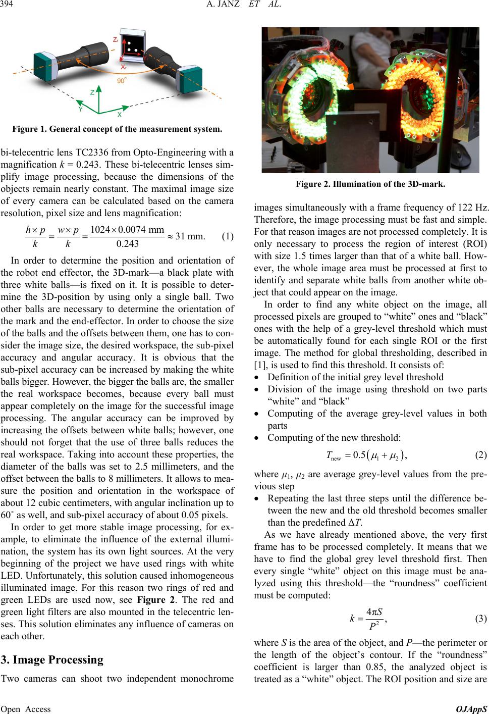 A. JANZ ET AL. 394 Figure 1. General concept of the measurement system. bi-telecentric lens TC2336 from Opto-Engineering with a magnification k = 0.243. These bi-telecentric lenses sim- plify image processing, because the dimensions of the objects remain nearly constant. The maximal image size of every camera can be calculated based on the camera resolution, pixel size and lens magnification: 10240.0074 mm31 mm. 0.243 hp wp kk (1) In order to determine the position and orientation of the robot end effector, the 3D-mark—a black plate with three white balls—is fixed on it. It is possible to deter- mine the 3D-position by using only a single ball. Two other balls are necessary to determine the orientation of the mark and the end-effector. In order to choose the size of the balls and the offsets between them, one has to con- sider the image size, the desired workspace, the sub-pixel accuracy and angular accuracy. It is obvious that the sub-pixel accuracy can be increased by making the white balls bigger. However, the bigger the balls are, the smaller the real workspace becomes, because every ball must appear completely on the image for the successful image processing. The angular accuracy can be improved by increasing the offsets between white balls; however, one should not forget that the use of three balls reduces the real workspace. Taking into account these properties, the diameter of the balls was set to 2.5 millimeters, and the offset between the balls to 8 millimeters. It allows to mea- sure the position and orientation in the workspace of about 12 cubic centimeters, with angular inclination up to 60˚ as well, and sub-pixel accuracy of about 0.05 pixels. In order to get more stable image processing, for ex- ample, to eliminate the influence of the external illumi- nation, the system has its own light sources. At the very beginning of the project we have used rings with white LED. Unfortunately, this solution caused inhomogeneous illuminated image. For this reason two rings of red and green LEDs are used now, see Figure 2. The red and green light filters are also mounted in the telecentric len- ses. This solution eliminates any influence of cameras on each other. 3. Image Processing Two cameras can shoot two independent monochrome Figure 2. Illumination of the 3D-mark. images simultaneously with a frame frequency of 122 Hz. Therefore, the image processing must be fast and simple. For that reason images are not processed completely. It is only necessary to process the region of interest (ROI) with size 1.5 times larger than that of a white ball. How- ever, the whole image area must be processed at first to identify and separate white balls from another white ob- ject that could appear on the image. In order to find any white object on the image, all processed pixels are grouped to “white” ones and “black” ones with the help of a grey-level threshold which must be automatically found for each single ROI or the first image. The method for global thresholding, described in [1], is used to find this threshold. It consists of: Definition of the initial grey level threshold Division of the image using threshold on two parts “white” and “black” Computing of the average grey-level values in both parts Computing of the new threshold: new1 2 0.5 ,T (2) where μ1, μ2 are average grey-level values from the pre- vious step Repeating the last three steps until the difference be- tween the new and the old threshold becomes smaller than the predefined ΔT. As we have already mentioned above, the very first frame has to be processed completely. It means that we have to find the global grey level threshold first. Then every single “white” object on this image must be ana- lyzed using this threshold—the “roundness” coefficient must be computed: 2 4π, S kP (3) where S is the area of the object, and P—the perimeter or the length of the object’s contour. If the “roundness” coefficient is larger than 0.85, the analyzed object is treated as a “white” object. The ROI position and size are Open Access OJAppS  A. JANZ ET AL. 395 then computed for it. Furthermore, only these ROIs will be processed. Figure 3 shows an example of the first frame. “White” objects found in ROIs will no longer be ana- lyzed with the “roundness” coefficient. The fitting to circle method is used in order to find the center of the circle on the image. First of all, a contour of the circle must be found. Only neighbor pixels are scanned to re- duce the processing time to a minimum. The scan runs clockwise until the contour is closed. This way the fol- lowing equation is true for every point of the contour (see Figure 4): 22 2, cc xyyR (4) where x and y are the coordinates of any contour point, xc and yc—the unknown coordinates of the circle center, R—the unknown radius of the circle. The Equation (4) can also be expressed as: Figure 3. Fragment of the first image. Figure 4. Fitting to the circle. 2222 2 22 cccc AB C xy xxyyxyR0, (5) or 22 . xByCx y (6) To use all points of the contour, Equation (6) is ex- pressed in the matrix form: 22 11 1111 22 22 2222 22 1 1 1 nn nnnn AxBy Cxy y A AxBy Cxy y B C AxBy Cxy y ABC XY Q (7) or YABCQ (8) The unknown matrix ABC can be computed with the help of the following equation: †,ABCXYQ (9) where (XY)† is the pseudo inverse matrix of the matrix XY. The coordinates of the circle center xc and yc can be easily found from the two first elements of the matrix ABC. 4. Camera Calibration To determine the position of the robot’s end-effector in a 3D-workspace it is not sufficient to have the 2D image coordinates of the balls measured by the two cameras. The 2D-data from the two cameras has to be fused to get the 3D-data. To do so, the relationship between the two cameras must be exactly determined. In order to find this relationship, it is necessary to carry out a measurement, in which the two cameras measure the image positions of a set of objects in the well-known 3D-position. Further- more, parameters of each camera which cause systematic measurement errors can also be determined in this meas- urement. This procedure is called camera matching and calibration. Various camera calibration methods were described in [2-4]. They are mostly based on the pin-hole camera model, where the 3D-points are projected to the image through a single point called camera center. The accuracy of the camera calibration can be increased if the distor- tion of the camera image, caused by lenses mounted on the camera is considered. Most popular models of the lens distortion can be found in [5-7]. The calibration of a multiple view camera system is more complex, because the intrinsic and extrinsic parameters of the single cam- era as well as the relationship (relative position and ori- entation) between two (or more) cameras must be found. Open Access OJAppS  A. JANZ ET AL. 396 Computation of the multiple view geometry is described in [8]. The description of the two view geometry can be found in [9-11]. 4.1. Camera Model The most often used and well-known camera model is the pin-hole camera model [8]. This model is described with the help of the projection matrix P of the camera: , PKRRC (10) where R is rotation matrix of the camera in the world coordinate system, C—coordinates of the camera center in the absolute coordinate system, K—the camera cali- bration matrix. The camera calibration matrix K includes parameters such as focal length f and position of the principal point , y pp in the coordinate system of the image . 1 x y p p K 0 , (11) The projection matrix P is used for triangulation and computing of the 3D-data from the 2D image data, be- cause it expresses the relationship between the world points W and their corresponding image points w: ,wPW (12) where and . T ,,1xyw T ,,,1XYZW 4.2. Independent Calibration As independent calibration of two cameras or simply independent calibration in this paper we have applied a calibration method, in which a set of 3D points with ex- act positions are shot with two cameras simultaneously. The projection matrix is then computed from the 3D world data and the 2D image. The 3D data can be recon- structed with help of the computed projection matrix and the image data of both cameras and the geometric recon- struction error can be found. If the reconstruction accu- racy does not satisfy the requirements of the measure- ment system, the projection matrices can be refined by iteratively minimizing the geometric reconstruction error (for example, Levenberg-Marquardt algorithm). The computation of initial projection matrices is based on the direct linear transformation (DLT). According to [8], for each correspondence Wi ↔ wi the following rela- tionship can be derived: TT 1 TT 2 TT 3 0 0 0 ii ii ii ii ii ii P A WyW P WxWP yW xWP ω ω (13) where are normalized image points, W—normalized 3D data, P1, P2 and P3—rows of projec- tion matrix P in a normalized form and i—index of the point. The projection matrix P can be found after having obtained the singular value decomposition (SVD) of the matrix A for all the given points. So if A = UDVT, then the solution is the last column of the matrix V. T ,,wxyω When projection matrices of both cameras are com- puted, the 3D world point can be reconstructed. For this purpose, the triangulation [8] from the corresponding image points w and w' of both cameras and projection matrices P and P' (also based on the DLT) is used: 0 0, 0 wPW AW wPW (14) where TT 31 TT 32 TT 31 TT 32 . xP P yP P A xP P yP P (15) The 3D data can be reconstructed with the help of the SVD of the matrix A by computing the projection matri- ces, like in the solution above. In order to minimize the geometric error, projection matrices must be refined using the Levenberg-Marquardt (LM) minimization method. For this purpose both pro- jection matrices are composed to an optimization matrix and the LM-algorithm runs until the geometric error reaches a minimum. Once the geometric error is minimized, the projection matrices stay constant for further measure- ments until some mechanical parameters (for example, camera orientation) are changed. 4.3. Fundamental and Essential Matrices In the previous chapter, the projection matrices were matched to each other with the help of the LM-algorithm in order to obtain the minimal reconstruction error. An- other method based on the computation of the funda- mental matrix, i.e. a matrix, which contains the relation- ship between two cameras, their extrinsic and intrinsic parameters. The fundamental matrix is defined by the equation T0, wFw (16) where F is fundamental matrix, w and w'—corresponding image points. From (16) it follows that the fundamental matrix can be computed when having only the corre- sponding image points. To do so, the (16) must be trans- formed to Open Access OJAppS 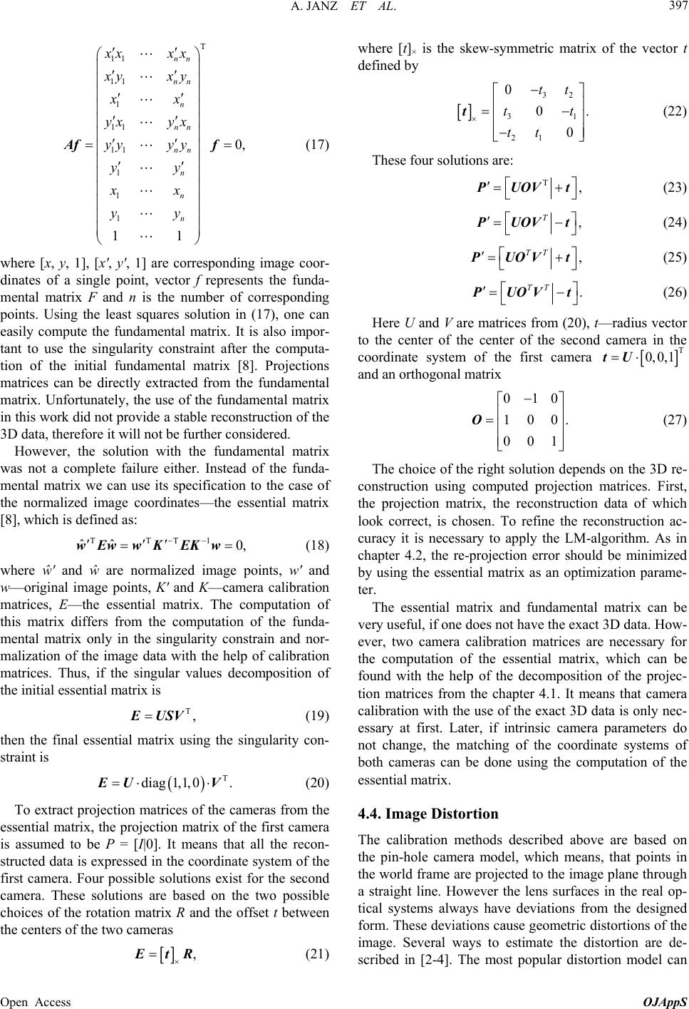 A. JANZ ET AL. 397 T 11 11 1 11 11 1 1 1 0, 11 nn nn n nn nn n n n xxx x xyx y xx yxyx yyyy yy xx yy Aff (17) where [x, y, 1], [x', y', 1] are corresponding image coor- dinates of a single point, vector f represents the funda- mental matrix F and n is the number of corresponding points. Using the least squares solution in (17), one can easily compute the fundamental matrix. It is also impor- tant to use the singularity constraint after the computa- tion of the initial fundamental matrix [8]. Projections matrices can be directly extracted from the fundamental matrix. Unfortunately, the use of the fundamental matrix in this work did not provide a stable reconstruction of the 3D data, therefore it will not be further considered. However, the solution with the fundamental matrix was not a complete failure either. Instead of the funda- mental matrix we can use its specification to the case of the normalized image coordinates—the essential matrix [8], which is defined as: TTT1 ˆˆ0, wEwwKEKw (18) where ŵ' and ŵ are normalized image points, w' and w—original image points, K' and K—camera calibration matrices, E—the essential matrix. The computation of this matrix differs from the computation of the funda- mental matrix only in the singularity constrain and nor- malization of the image data with the help of calibration matrices. Thus, if the singular values decomposition of the initial essential matrix is T, USV (19) then the final essential matrix using the singularity con- straint is T diag1,1, 0. UV (20) To extract projection matrices of the cameras from the essential matrix, the projection matrix of the first camera is assumed to be P = [I|0]. It means that all the recon- structed data is expressed in the coordinate system of the first camera. Four possible solutions exist for the second camera. These solutions are based on the two possible choices of the rotation matrix R and the offset t between the centers of the two cameras , tR (21) where [t]× is the skew-symmetric matrix of the vector t defined by 32 3 21 0 0 0 tt t tt 1 .t t (22) These four solutions are: T, PUOVt (23) , T PUOVt (24) , TT PUOV t (25) . TT PUOVt (26) Here U and V are matrices from (20), t—radius vector to the center of the center of the second camera in the coordinate system of the first camera and an orthogonal matrix T 0, 0,1tU 010 100 001 . O (27) The choice of the right solution depends on the 3D re- construction using computed projection matrices. First, the projection matrix, the reconstruction data of which look correct, is chosen. To refine the reconstruction ac- curacy it is necessary to apply the LM-algorithm. As in chapter 4.2, the re-projection error should be minimized by using the essential matrix as an optimization parame- ter. The essential matrix and fundamental matrix can be very useful, if one does not have the exact 3D data. How- ever, two camera calibration matrices are necessary for the computation of the essential matrix, which can be found with the help of the decomposition of the projec- tion matrices from the chapter 4.1. It means that camera calibration with the use of the exact 3D data is only nec- essary at first. Later, if intrinsic camera parameters do not change, the matching of the coordinate systems of both cameras can be done using the computation of the essential matrix. 4.4. Image Distortion The calibration methods described above are based on the pin-hole camera model, which means, that points in the world frame are projected to the image plane through a straight line. However the lens surfaces in the real op- tical systems always have deviations from the designed form. These deviations cause geometric distortions of the image. Several ways to estimate the distortion are de- scribed in [2-4]. The most popular distortion model can Open Access OJAppS 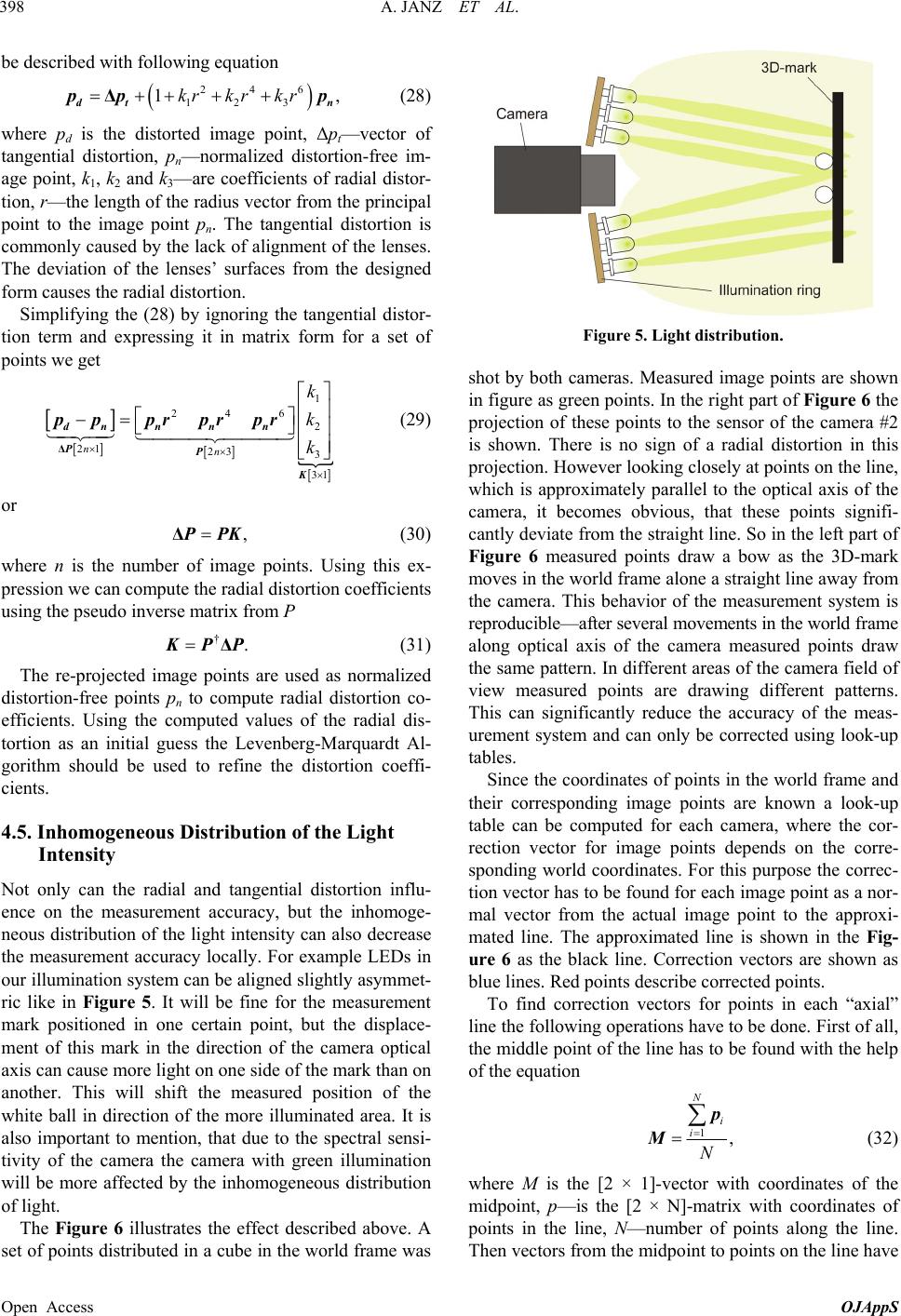 A. JANZ ET AL. 398 be described with following equation 246 123 1,krk rkr dt pp pΔn (28) where pd is the distorted image point, Δpt—vector of tangential distortion, pn—normalized distortion-free im- age point, k1, k2 and k3—are coefficients of radial distor- tion, r—the length of the radius vector from the principal point to the image point pn. The tangential distortion is commonly caused by the lack of alignment of the lenses. The deviation of the lenses’ surfaces from the designed form causes the radial distortion. Simplifying the (28) by ignoring the tangential distor- tion term and expressing it in matrix form for a set of points we get 1 246 2 21 23 3 31 nn k k k dn n n n PP K p pprprpr Δ (29) or ,PPKΔ (30) where n is the number of image points. Using this ex- pression we can compute the radial distortion coefficients using the pseudo inverse matrix from P †. PPΔ (31) The re-projected image points are used as normalized distortion-free points pn to compute radial distortion co- efficients. Using the computed values of the radial dis- tortion as an initial guess the Levenberg-Marquardt Al- gorithm should be used to refine the distortion coeffi- cients. 4.5. Inhomogeneous Distribution of the Light Intensity Not only can the radial and tangential distortion influ- ence on the measurement accuracy, but the inhomoge- neous distribution of the light intensity can also decrease the measurement accuracy locally. For example LEDs in our illumination system can be aligned slightly asymmet- ric like in Figure 5. It will be fine for the measurement mark positioned in one certain point, but the displace- ment of this mark in the direction of the camera optical axis can cause more light on one side of the mark than on another. This will shift the measured position of the white ball in direction of the more illuminated area. It is also important to mention, that due to the spectral sensi- tivity of the camera the camera with green illumination will be more affected by the inhomogeneous distribution of light. The Figure 6 illustrates the effect described above. A set of points distributed in a cube in the world frame was Figure 5. Light distribution. shot by both cameras. Measured image points are shown in figure as green points. In the right part of Figure 6 the projection of these points to the sensor of the camera #2 is shown. There is no sign of a radial distortion in this projection. However looking closely at points on the line, which is approximately parallel to the optical axis of the camera, it becomes obvious, that these points signifi- cantly deviate from the straight line. So in the left part of Figure 6 measured points draw a bow as the 3D-mark moves in the world frame alone a straight line away from the camera. This behavior of the measurement system is reproducible—after several movements in the world frame along optical axis of the camera measured points draw the same pattern. In different areas of the camera field of view measured points are drawing different patterns. This can significantly reduce the accuracy of the meas- urement system and can only be corrected using look-up tables. Since the coordinates of points in the world frame and their corresponding image points are known a look-up table can be computed for each camera, where the cor- rection vector for image points depends on the corre- sponding world coordinates. For this purpose the correc- tion vector has to be found for each image point as a nor- mal vector from the actual image point to the approxi- mated line. The approximated line is shown in the Fig- ure 6 as the black line. Correction vectors are shown as blue lines. Red points describe corrected points. To find correction vectors for points in each “axial” line the following operations have to be done. First of all, the middle point of the line has to be found with the help of the equation 1, N i i N p M (32) where M is the [2 × 1]-vector with coordinates of the midpoint, p—is the [2 × N]-matrix with coordinates of points in the line, N—number of points along the line. Then vectors from the midpoint to points on the line have Open Access OJAppS 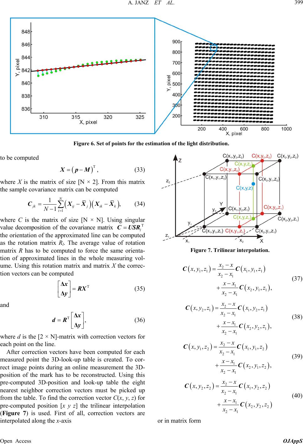 A. JANZ ET AL. Open Access OJAppS 399 Figure 6. Set of points for the estimation of the light distribution. to be computed T,XpM (33) where X is the matrix of size [N × 2]. From this matrix the sample covariance matrix can be computed 1 1, 1 N jkijjikk i N CXXX X (34) where C is the matrix of size [N × N]. Using singular value decomposition of the covariance matrix the orientation of the approximated line can be computed as the rotation matrix Rl. The average value of rotation matrix R has to be computed to force the same orienta- tion of approximated lines in the whole measuring vol- ume. Using this rotation matrix and matrix X the correc- tion vectors can be computed T l CUSR Figure 7. Trilinear interpolation. 2 111 11 21 1 211 21 ,, ,, ,, , xx xy zx y z xx xx yz xx CC C (37) T xRX y Δ Δ (35) 2 211 21 21 1 221 21 ,, ,, ,, , xx xy zxy z xx xx yz xx CC C (38) and T, x dR Δ Δ (36) where d is the [2 × N]-matrix with correction vectors for each point on the line. 2 12 112 21 1 212 21 ,, ,, ,,, xx xy zx y z xx xx yz xx CC C (39) After correction vectors have been computed for each measured point the 3D-look-up table is created. To cor- rect image points during an online measurement the 3D- position of the mark has to be reconstructed. Using this pre-computed 3D-position and look-up table the eight nearest neighbor correction vectors must be picked up from the table. To find the correction vector C(x, y, z) for pre-computed position [x y z] the trilinear interpolation (Figure 7) is used. First of all, correction vectors are interpolated along the x-axis 2 22 122 21 1 222 21 ,, ,, ,, xx yz xyz xx xx yz xx CC C (40) or in matrix form 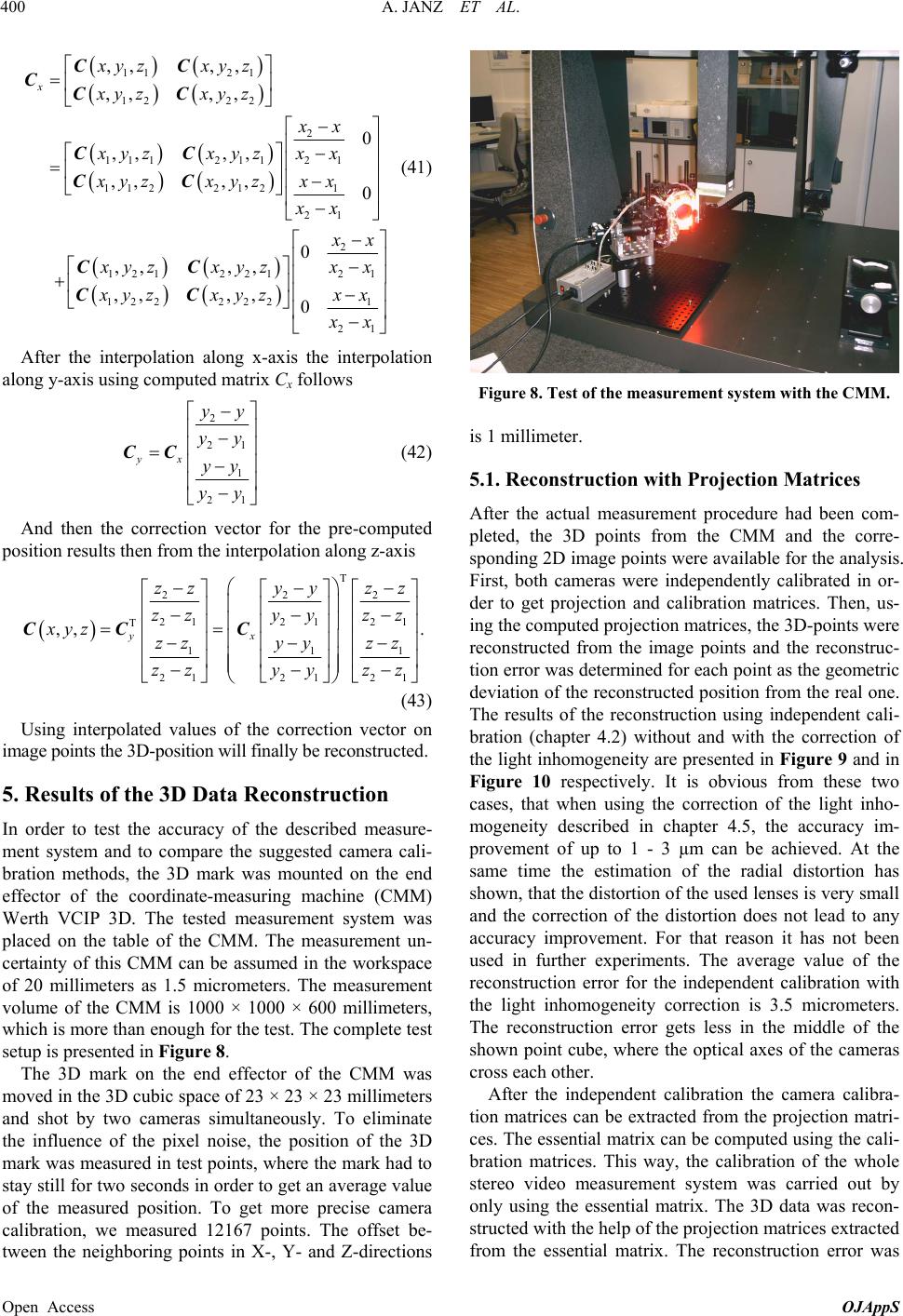 A. JANZ ET AL. 400 11 21 12 22 2 21 111 211 112 2121 21 2 21 121 221 122 2221 21 ,,, , ,, ,, 0 ,, ,, ,, ,,0 0 ,, ,, ,,,,0 x xy zxyz xy zxyz xx xx xyzxyz xyzxyzxx xx x x xyzx yz xyzx yz x x CC CCC CC CC CC CC (41) After the interpolation along x-axis the interpolation along y-axis using computed matrix Cx follows 2 21 1 21 yx yy yy yy yy CC (42) And then the correction vector for the pre-computed position results then from the interpolation along z-axis T 222 212121 T 11 212121 ,, . yx zzyy zz zzyy zz xyz zzyy zz zzyy zz CCC 1 (43) Using interpolated values of the correction vector on image points the 3D-position will finally be reconstructed. 5. Results of the 3D Data Reconstruction In order to test the accuracy of the described measure- ment system and to compare the suggested camera cali- bration methods, the 3D mark was mounted on the end effector of the coordinate-measuring machine (CMM) Werth VCIP 3D. The tested measurement system was placed on the table of the CMM. The measurement un- certainty of this CMM can be assumed in the workspace of 20 millimeters as 1.5 micrometers. The measurement volume of the CMM is 1000 × 1000 × 600 millimeters, which is more than enough for the test. The complete test setup is presented in Figure 8. The 3D mark on the end effector of the CMM was moved in the 3D cubic space of 23 × 23 × 23 millimeters and shot by two cameras simultaneously. To eliminate the influence of the pixel noise, the position of the 3D mark was measured in test points, where the mark had to stay still for two seconds in order to get an average value of the measured position. To get more precise camera calibration, we measured 12167 points. The offset be- tween the neighboring points in X-, Y- and Z-directions Figure 8. Test of the measurement system with the CMM. is 1 millimeter. 5.1. Reconstruction with Projection Matrices After the actual measurement procedure had been com- pleted, the 3D points from the CMM and the corre- sponding 2D image points were available for the analysis. First, both cameras were independently calibrated in or- der to get projection and calibration matrices. Then, us- ing the computed projection matrices, the 3D-points were reconstructed from the image points and the reconstruc- tion error was determined for each point as the geometric deviation of the reconstructed position from the real one. The results of the reconstruction using independent cali- bration (chapter 4.2) without and with the correction of the light inhomogeneity are presented in Figure 9 and in Figure 10 respectively. It is obvious from these two cases, that when using the correction of the light inho- mogeneity described in chapter 4.5, the accuracy im- provement of up to 1 - 3 µm can be achieved. At the same time the estimation of the radial distortion has shown, that the distortion of the used lenses is very small and the correction of the distortion does not lead to any accuracy improvement. For that reason it has not been used in further experiments. The average value of the reconstruction error for the independent calibration with the light inhomogeneity correction is 3.5 micrometers. The reconstruction error gets less in the middle of the shown point cube, where the optical axes of the cameras cross each other. After the independent calibration the camera calibra- tion matrices can be extracted from the projection matri- ces. The essential matrix can be computed using the cali- bration matrices. This way, the calibration of the whole stereo video measurement system was carried out by only using the essential matrix. The 3D data was recon- structed with the help of the projection matrices extracted from the essential matrix. The reconstruction error was Open Access OJAppS  A. JANZ ET AL. 401 Figure 9. Reconstruction using the independent calibration. Figure 10. Reconstruction using the independent calibration and light inhomogeneity correction. analyzed in the way described above. The results of the reconstruction using calibration with the essential matrix (chapter 4.3) are presented in Figure 11—without light inhomogeneity correction and in Figure 12—with light inhomogeneity correction. Similar to the experiment with the independent calibration the light inhomogeneity cor- rection improves accuracy of the system in case of the essential matrix method up to 0.5 - 2 µm. The average value of the reconstruction error for this method is 0.05 micrometers. Like in the previous method the reconstruc- tion error gets less in the middle of the points cube, but the distribution of this error in the workspace is much steadier. It is obvious that the reconstruction results become much more accurate after the system has been calibrated using the essential matrix. It can be explained by the fact that the essential matrix describes not only the intrinsic parameters but also the position and orientation of both cameras relatively to each other. Unlike it, a simple in- dependent computation of the projection matrices only describes the relationship between the world points and the camera image. Therefore, the calibration with the Figure 11. Reconstruction using the essential matrix. Figure 12. Reconstruction using the essential matrix and the light inhomogeneity correction. essential matrix can better match the coordinate systems of the two cameras than the independent calibration. 5.2. Affine Reconstruction In respect to the fact that both cameras have telecentric lenses, their camera models can be approximated to the affine camera model—all projection lines are assumed to be parallel to each other and the last row of the projection matrix has the form (0, 0, 0, 1). Using this assumption, the affine reconstruction can be implemented to get the 3D data from the corresponding image points. The re- construction can be carried out with the help of the fac- torization algorithm described in [8] (the algorithm 18.1). First of all, the origin of every image must be translated to the center of points in this image. The translation vec- tor t for the camera with the index i is then 1 1, n ii j n tw (44) where wi are points on the image i, j—index of the point, n—number of points on the image. The translation is de- Open Access OJAppS  A. JANZ ET AL. 402 fined by the equation ˆ, ii i wwmt (45) where wi are original image points in the image i, ŵi—new or translated points in the image i, m—the vec- tor of size [n × 1], all the elements of which are equal 1. Then the measurement matrix M of size [4 × n] is composed from the new image coordinates ŵi: 11 1 12 22 2 12 ˆˆˆ . ˆˆˆ n n ww w Mww w (46) Then from its SVD M = UDVT the 3D normalized points are obtained from the first three columns of V. As described above, the affine reconstruction was tested using the same measurement data as used in chap- ter 5.1; the geometric reconstruction error was analyzed as well. The results of the affine reconstruction are pre- sented in Figure 13—without the light inhomogeneity correction and in Figure 14—with the light inhomogene- ity correction. The average value of the reconstruction error for this method is approximately 3.25 micrometers. Unlike the reconstruction using the independent cali- bration and essential matrix, the affine reconstruction does not require the computation of the camera projec- tion matrices. The reconstruction occurs directly from the image data; at least four corresponding points are re- quired though. However, this reconstruction method can- not be used for an online-measurement of the 3D-posi- tion due to the computation effort caused by a large data volume. 6. Conclusions The reconstruction results and the measurement accuracy can be analyzed more carefully. Figure 15 depicts a dis- tribution of the reconstruction error for all the three de- scribed methods. Here the whole error area is divided into 50 intervals. The number of points with the recon- struction error is found in every interval and then pre- sented as point-marks on the graphic. The average value of the error for all point is presented as a line. It is obvi- ous from the figure that the distribution of the recon- struction error is similar to the affine reconstruction and the reconstruction using independent calibration. The distribution of the error for the reconstruction using the essential matrix is very small in comparison to the other two methods. Furthermore, the average value of the re- construction error in case of the essential matrix is sig- nificantly smaller than in the other two cases. Therefore, the calibration using the essential matrix will be used for the calibration of the system as the standard method. The independent calibration will be only used to compute the initial values of the calibration matrices if the intrinsic parameters have somehow changed. Figure 13. Affine reconstruction. Figure 14. Affine reconstruction using correction of the light inhomogeneity. Figure 15. Distribution of the reconstruction error. Note that in order to estimate the accuracy of the measurement system, the image processing accuracy of 1.5 micrometers (the pixel noise was strongly suppressed for the calibration measurement) must be added to the reconstruction error. Thus, if the average value of the reconstruction error using essential matrix is about 0.05 micrometers, the accuracy of the measurement system is 1.55 micrometers. Open Access OJAppS  A. JANZ ET AL. Open Access OJAppS 403 REFERENCES [1] R. C. Gonzalez and R. E. Woods, “Digital Image Proc- essing,” 2nd Edition, Prentice Hall, Upper Saddle River, 2002. [2] J. Heikkilä, “Geometric Camera Calibration Using Circu- lar Control Points,” IEEE Transaction on Pattern Analy- sis and Machine Intelligence, Vol. 22, No. 10, 2000, pp. 1066-1077. http://dx.doi.org/10.1109/34.879788 [3] Z. Zhang, “Flexible Camera Calibration by Viewing a Plane from Unknown Orientations,” Proceedings of the International Conference on Computer Vision ICCV, Ker- kyra, 20-27 September 1999, pp. 666-673. http://dx.doi.org/10.1109/ICCV.1999.791289 [4] R. Y. Tsai, “A Versatile Camera Calibration Technique for High-Accuracy 3D Machine Vision Metrology Using Off-the-Shelf TV Cameras and Lenses,” IEEE Journal of Robotics and Automation, Vol. 3, No. 4, 1987, pp. 323- 344. http://dx.doi.org/10.1109/JRA.1987.1087109 [5] C. Ricolfe-Viala and A.-J. Sanches-Salmeron, “Lens Dis- tortion Models Evaluation,” Applied Optics, Vol. 49, No. 30, 2012, pp. 5914-5928. http://dx.doi.org/10.1364/AO.49.005914 [6] Z. Zhang, “A Flexible New Technique for Camera Cali- bration,” IEEE Transaction on Pattern Analysis and Ma- chine Intelligence, Vol. 22, No. 11, 2000, pp. 1330-1334. http://dx.doi.org/0.1109/34.888718 [7] R. Hartley and S. B. Kang, “Parameter-free Radial Dis- tortion Correction with Centre of Distortion Estimation,” Proceeding of the 10th IEEE International Conference on Computer Vision ICCV’05, Beijing, 17-21 October 2005, pp. 1-8. [8] R. Hartley and A. Zisserman, “Multiple View Geometry in Computer Vision,” 2nd Edition, Cambridge University Press, Cambridge, 2003. [9] R. Hartley and C. Silpa-Anan, “Reconstruction from Two Views Using Approximate Calibration,” Proceedings of the 5th Asian Conference on Computer Vision ACCV’02, Melbourne, January 2004, pp. 1-6. [10] B. Albouy, S. Treuillet, Y. Lucas and D. Birov, “Funda- mental Matrix Estimation Revisited Through a Global 3D Reconstruction Framework,” Proceedings of the Advanced Concepts for Intelligent Vision Systems ACIVS 2004, Brus- sels, 31 August-3 September 2004, pp. 185-192. [11] K. Kanatani and Y. Sugaya, “Compact Fundamental Ma- trix Computation,” Proceedings of the 3rd Pacific Rim Sym- posium of Image and Video Technology, Tokyo, 13-16 January 2009, pp. 179-190.
|