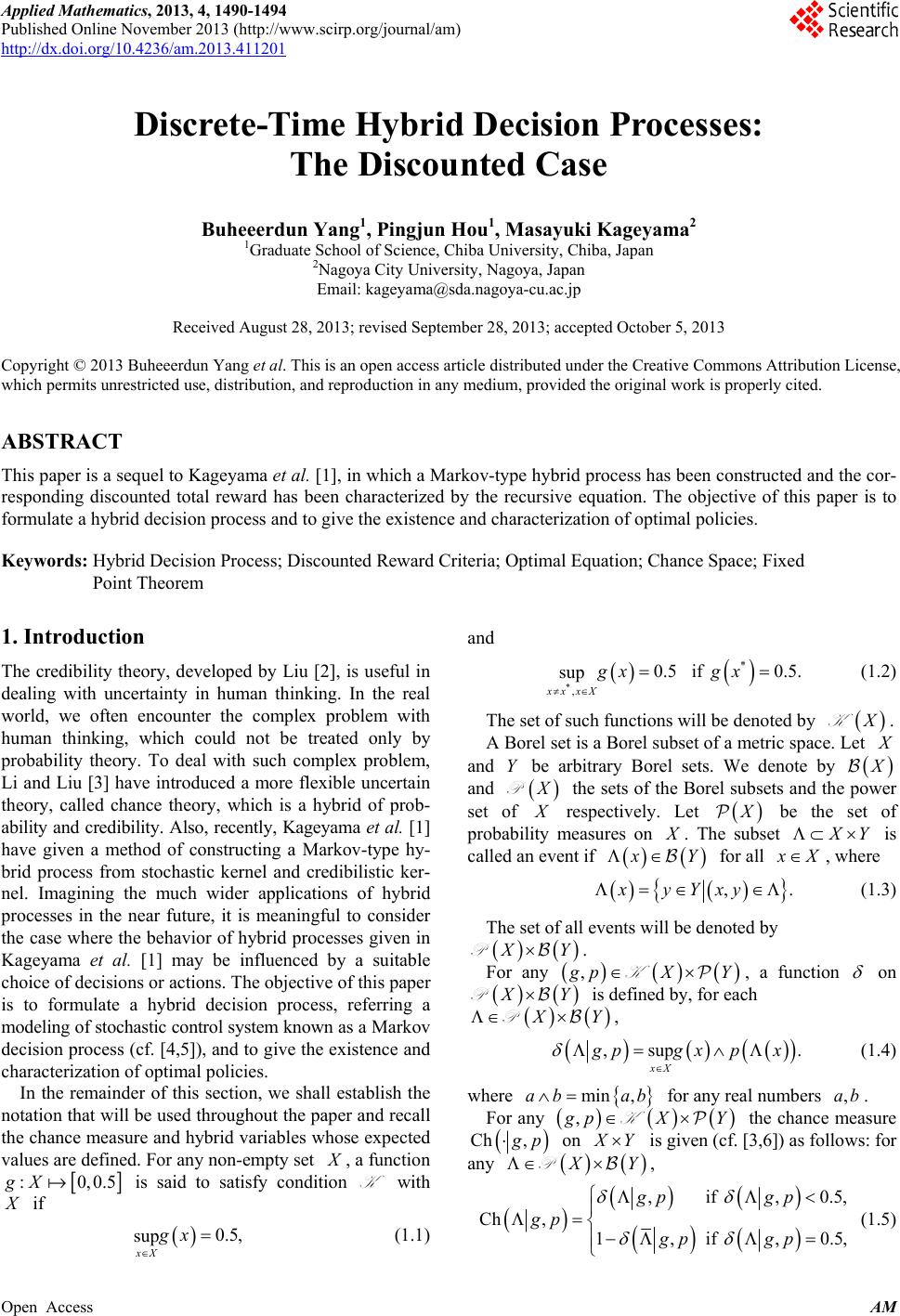
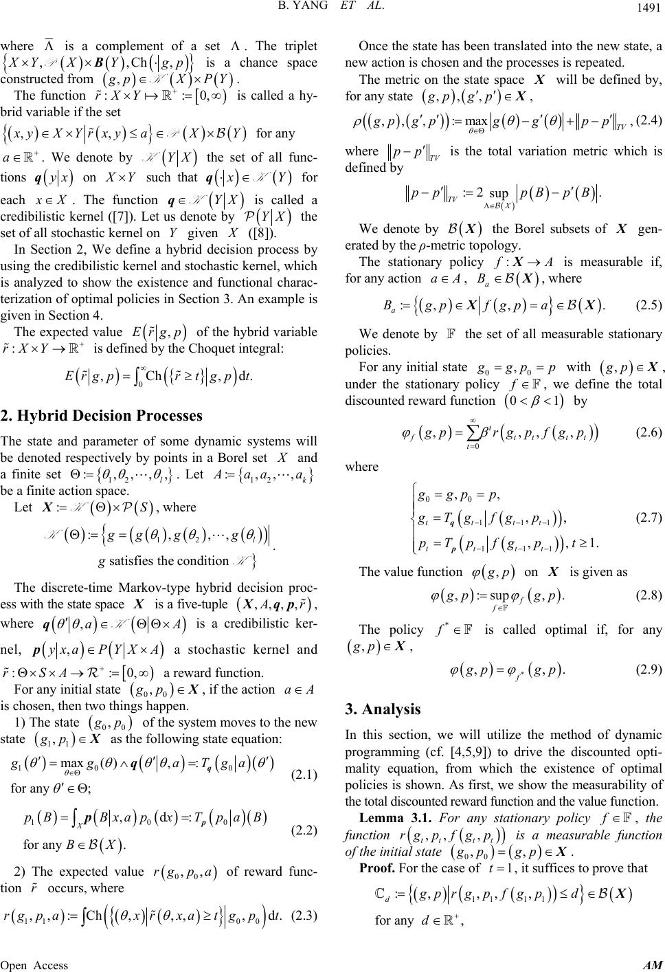
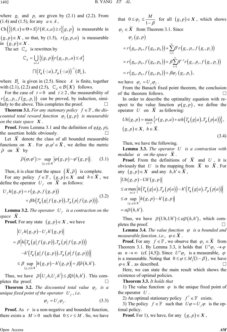
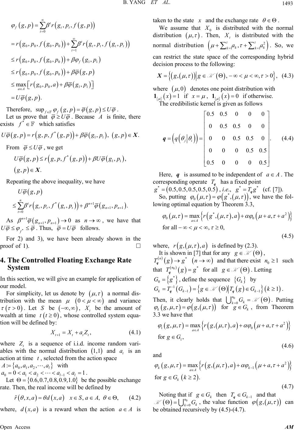
 Applied Mathematics, 2013, 4, 1490-1494 Published Online November 2013 (http://www.scirp.org/journal/am) http://dx.doi.org/10.4236/am.2013.411201 Open Access AM Discrete-Time Hybrid Decision Processes: The Discounted Case Buheeerdun Yang1, Pingjun Hou1, Masayuki Kageyama2 1Graduate School of Science, Chiba University, Chiba, Japan 2Nagoya City University, Nagoya, Japan Email: kageyama@sda.nagoya-cu.ac.jp Received August 28, 2013; revised September 28, 2013; accepted October 5, 2013 Copyright © 2013 Buheeerdun Yang et al. This is an open access article distributed under the Creative Commons Attribution License, which permits unrestricted use, distribution, and reproduction in any medium, provided the original work is properly cited. ABSTRACT This paper is a sequel to Kageyama et al. [1], in which a Markov-type hybrid process has been constructed and the cor- responding discounted total reward has been characterized by the recursive equation. The objective of this paper is to formulate a hybrid decision process and to give the existence and characterization of optimal policies. Keywords: Hybrid Decision Process; Discounted Reward Criteria; Optimal Equation; Chance Space; Fixed Point Theorem 1. Introduction The credibility theory, developed by Liu [2], is useful in dealing with uncertainty in human thinking. In the real world, we often encounter the complex problem with human thinking, which could not be treated only by probability theory. To deal with such complex problem, Li and Liu [3] have introduced a more flexible uncertain theory, called chance theory, which is a hybrid of prob- ability and credibility. Also, recently, Kageyama et al. [1] have given a method of constructing a Markov-type hy- brid process from stochastic kernel and credibilistic ker- nel. Imagining the much wider applications of hybrid processes in the near future, it is meaningful to consider the case where the behavior of hybrid processes given in Kageyama et al. [1] may be influenced by a suitable choice of decisions or actions. The objective of this paper is to formulate a hybrid decision process, referring a modeling of stochastic control system known as a Mar k ov decision process (cf. [4,5]), and to give the existence and characterization of optimal policies. In the remainder of this section, we shall establish the notation that will be used throughout the paper and recall the chance measure and hybrid variables whose expected values are d efined. Fo r an y no n- empty set , a function :0,0.gX5 is said to satisfy condition with K if 0.5, sup xX gx (1.1) and * * , 0.5 if0.5. sup xx xX gx gx (1.2) The set of such functions will be denoted by K. A Borel set is a Borel subset of a metric space. Let and be arbitrary Borel sets. We denote by Y and P the sets of the Borel subsets and the power set of respectively. Let be the set of probability measures on . The subset Y is called an event if Y for all X, where ,xyYxy. (1.3) The set of all events will be denoted by YP. For any , pXKY, a function on YP is defined by, for each YP, ,. sup xX pgxpx (1.4) where min ,ab ab for any real numbers . ,ab For any , pXKY the chance measure Ch , p on Y is given (cf. [3,6]) as follows: for any YP, ,if,0 Ch ,1,if, gp gp gp gp gp .5, 0.5, (1.5)  B. YANG ET AL. 1491 where is a complement of a set . The triplet ,,Ch , YX Ygp BP is a chance space constructed from , pXK ::rX Y PY 0, . The function is called a hy- brid variable if the set ,, yXYrxyaXY P for any a . We denote by YXK the set of all func- tions yx q on Y such that YqK for each X. The function YXqK is called a credibilistic kernel ([7]). Let us denote by YX the set of all stochastic kernel on given Y ([8]). In Section 2, We define a hybrid decision process by using the credibilistic k ernel and stochastic kernel, wh ich is analyzed to show the existence and functional charac- terization of optimal policies in Sectio n 3. An example is given in Section 4. The expected value ,Ergp of the hybrid variable is defined by the Choquet in t e gral : :rX Y 0 ,Ch ,Ergprt gpt d. 2. Hybrid Decision Processes The state and parameter of some dynamic systems will be denoted respectively by points in a Borel set and a finite set 12 :,,,, l . Let , 12 :, , k aa a be a finite action space. Let , where :SXK 12 :,,, satisfies the condition l gg gg g K K . The discrete-time Markov-type hybrid decision proc- ess with the state space is a five-tuple ,,,, r qp, where , A qKa is a credibilistic ker- nel, ,yxaPY XAp 0, a stochastic kernel and ::rSA ,gp a reward function. For any initial state 00 , if the action aA is chosen, then two things happen. 1) The state 00 , p of the system moves to the new state 11 ,gp as the following state equation: 10 0 max(),: for any; gg aTga q q (2.1) 10 ,d: for any. X pBBxapxT paB BX p p 0 (2.2) 2) The expected value of reward func- tion occurs, where 00 ,,rgp a r 110 0 ,,:Ch,,,, d.rgpaxrxat gpt (2.3) Once the state has been translated into the new state, a new action is chosen and the processes is repeated. The metric on the state space will be defined by, for any state ,,,gpgp , ,,, :max, TV gpg pggpp (2.4) where TV pp is the total variation metric which is defined by :2 . sup TV X pppBpB We denote by the Borel subsets of gen- erated by the ρ-metric topology. The stationary policy is measurable if, for any action :fXA aA , a B , where :, , a Bgp fgpa . X (2.5) We denote by the set of all measurable stationary policies. For any initial state 00 , gp p with ,gp , under the stationary policy , we define the total discounted reward function by f 0 1 , tt 0 ,,, t ftt t prgpfgp (2.6) where 00 111 111 ,, ,, ,, tttt tttt ggpp gTg fgp pTp fgpt 1. q p (2.7) The value function , p on is given as ,:sup , f f . pg p (2.8) The policy * f is called optimal if, for any ,gp , * , f ,. pg p (2.9) 3. Analysis In this section, we will utilize the method of dynamic programming (cf. [4,5,9]) to drive the discounted opti- mality equation, from which the existence of optimal policies is shown. As first, we show the measurability of the total discounted reward function and the value function. Lemma 3.1. For any stationary policy f , the function ,,, tt tt rg pfgp is a measurable function of the initial state 00 ,gp ,gp . Proof. For the case of 1t , it suffices to prove that 11 11 :, ,,, for any, dgp rgpf gpd d Open Access AM  B. YANG ET AL. 1492 where 1 and 1 are given by (2.1) and (2.2). From (1.4) and (1.5), for any , p Aa Ch,, ,, Srxatgp is measurable in ,gp , so that, by (1.5), is measurable in ,,rgpa ,gp . The set is rewritten by d 11 1 ,,, |, | d aA a, prg pad TaTa qp where a is given in (2.5). Since is finite, together with (2.1), (2.2 ) and (2. 5) , d 2t follows. For the case of and , the measurability of can be proved, by induction, simi- larly to the above. This completes the proof. 0t t ,, , tt t rg pfg p Theorem 3.1. For any stationary policy , the dis- counted total reward function f , f p is measurable on the state space . Proof. From Le mma 3.1 and the definition of φf(g, p), the assertion holds obviously. Let denote the class of all bounded measurable functions on . For , , we define the metric on by , ,:,, sup gp . pgp X (3.1) Then, it is clear that the space , X is complete. For any policy , f ,gp and h , we define the operator U on as follows: ,,,, ,, , f Uhgprgpf gp hTgf gpTpf gp qp . (3.2) Lemma 3.2. The operator U is a contraction on the space . Proof. For any state ,gp , we have , ,, ,, , ,, , ,, , sup ff gp UhgpUhgp hTgf gpTpfgp hT gfgpTpfgp hgphgphh . qp qp X Thus, we have , ff UhUh hh , . This com- pletes the proof. Theorem 3.2. The discounted total value is a unique fixed point of the operator U, i.e. . ff U (3.3) Proof. As is a non-negative and bounded func tion, there exists a such that . So, we have r M00rM that 01 f for all ,gp , which shows f from Theorem 3.1. Since 00 001 1 00 001 00 0011 , ,,,,, , ,,,,, , ,,,,, f t tt tt t t tt tt t f gp rgpfgprg pf gp rgpfgprgpfgp rg p fg pgp we have ff U . From the Banach fixed point theorem, the conclusion of the theorem follows. In order to describe the optimality equation with re- spect to the value function , p , we define the operator on U as following: ,max,,, ,,. aA Uh g prg pahTgaTpa gp h qp XX , (3.4) Then, we have the following. Lemma 3.3. The operator is a contra ction with modulus U on the spa ce . Proof. From the definitions of and U, it is obviously that is the mapping from U to . For any ,gp and any ,hh , , ,, max ,, ,, sup ,. aA gp UhgpUhgp hTga TpahTga Tpa hgph gp hh qp qp X Thus, we have ,Uh Uhhh , , which com- pletes the proof. Lemma 3.4. The value function is a bounded and measurable function. i.e., . Proof. For any f , we observe that f from Theorem 3.1. By Lemma 3.3, it holds that n f U as (cf. [4,5]). Since n n U is a measurable, is a measurable. Noting that 01M , we have , as described. Here, we can state the main result which shows the existence of optimal policies. Theorem 3.3. It holds that 1) The value function is the unique fixed point of the operator . U 2) An optimal stationary policy exists. * f 3) The policy f such that UU is the op- timal policy. Proof. For 1), we have, fo r a ny ,gp , Open Access AM  B. YANG ET AL. 1493 0 0000 =1 00 0011 00 00 00 11 ,,,, ,,,,, , ,, ,, ,, ,, max,,, ,. t ftt t t tt tt t f aA gprgp f gp rgpfgprgpfgp rg p fg pgp rg p fg pgp rgp ag p Ugp Therefore, sup ,, ff pgpU . Let us prove that U . Because is finite, there exists which satisfies * f *11 ,,,, ,,,Ugprgpfgpgp gp . From U , we get *11 ,,,, , ,. Ugprgpfgp Ugp gp X , Repeating the above inequality, we have *1 11 0 , ,,,, . ntn ttttn n t Ugp rg p fg pgp As 111 ,0 n nn gp as , we have that n * f U . Thus, U follows. For 2) and 3), we have been already shown in the proof of 1). 4. The Controlled Floating Exchange Rate System In this section, we will give an example for application of our model. For simplicity, let us denote by , a normal dis- tribution with the mean 0 and variance . Let be , t 0 S, be the amount of wealth at time , whose controlled system equa- tion will be defined by: 0 tt 1, tttt XaZ (4.1) where t is a sequence of i.i.d. income random vari- ables with the normal distribution and is an action at time , selected from the action space 1,1 t a t 2 , , , l01 :, aa 01 aa a a 2 a with . 1 01 ll aa Let 0. 7,0.86,0.,0.9,1.0 be the possible excha ng e rate. Then, the real income will be defined by ,,,,,,rxa dxaxSaA where, is a reward when the action (4.2) ,dxa aA is the stattaken toe and the exchange rate . We assume tha0 t is distributed withnorm the al distribution , . Then, t X is distributed with the normal distrn ibutio 2 ,t kk aa . So, we 1 t k 1k ndican restrict the state sng hybrid pace of the correspo decision process to the following: , 0 ,, ,gg XK, (4.3) where ,0 des one point distribution with note x 1 1 if , 0x 1 if otherwise. ibiliss follows The credtic kernel is given a 0.5 0.5000 00.50.50 000.50.5 0000.5 0.5 000 ji q 0 . 0 0.5 0.5 f aA q (4.4) Here, is assed to be independent o q um . The corresponing operate Tq has a fixed point d *0.5,0.5,0.5,0 .5 ,0.5g, i.e., ** Tgq (cf. [7]). So, putting , * g 0,, , we have the fol- lowing optimal3, eqution by Theorem 3.a 00 ,m for all,0, a * ,,,rg a2 (4.5) where, ax aA ,a ,,rg a is defined by (2.3). , It is shown in [7] that for any gK, * ng g T q n and tha0 nt there exist 1 such that 0 n Tg * g q for all gK. Letting g * 0 Gthe sequeby , definence k G 11 GgT G 1 k k 1 GT kk g K . P qq . Then, it clearly holds that u 0 0 n k kG Ktting ,,,, kgg for k G, from Theorem 3.3 we have that 2 10 1 ,, , for , ,, max, aA rg aa gG a (4.6) and 2 1 m,, , for 2 kk aA k rgaa gGk ax . g ,,g , a (4.7) Noting that if k G then an 1k TG q nction d that 0 0 nG value fu ,,g k k K, the ca vely by (4.5)-(4. 7). n be obtained recursi Open Access AM  B. YANG ET AL. Open Access AM 1494 [1] M. KageyamaDiscrete-Tim /10.1007/s10700-011-9109-2 REFERENCES , B. Yang and P. Hou, “e Hy- brid Processes and Discounted Total Expected Values,” Fuzzy Optimization Decision Making, Vo l . 10, N o . 4, 2011, pp. 341-355. http://dx.doi.org ger-Verlag ce Measure for Hybrid Even -008-0308-x [2] B. Liu, “Uncertain Theory,” 2nd Edition, Sprin, Berlin, 2007. [3] X. Li and B. Liu, “Chants with Fuzziness and Randomness,” Soft Computing, Vol. 13, No. 2, 2009, pp. 105-115. http://dx.doi.org/10.1007/s00500 crete-Time[4] O. Hernandez-Lerma and J. B. Lasserre, “Dis Markov Control Processes, Basic Optimality Criteria,” Springer, New York, 1996. http://dx.doi.org/10.1007/978-1-4612-0729-0 [5] M. Puterman, “Markov and Sons, Inc., 1994. Decision Processes,” John Wiley http://dx.doi.org/10.1002/9780470316887 [6] B. Liu, “Uncertain Theory,” 3rd Edition, UTLAB, 2009. [7] M. Kageyama and K. Iwamura, “Discrete Time Credi- bilistic Processes: Construction and Convergences,” In- formation Sciences, Vol. 179, No. 24, 2009, pp. 4277- ob, “Stochastic Processes,” John Wiley, New York, amming,” Princeton Uni- versity Press, Princeton, 1957. 4283. [8] J. L. Do 1953. [9] R. E. Bellman, “Dynamic Progr
|