 Applied Mathematics, 2013, 4, 1485-1489 Published Online November 2013 (http://www.scirp.org/journal/am) http://dx.doi.org/10.4236/am.2013.411200 Open Access AM On Expressing the Probabilities of Categorical Responses as Linear Functions of Covariates Tejas A. Desai The Adani Institute of Infrastructure Management, Ahmedabad, India Email: tejasdesai4@gmail.com Received August 22, 2013; revised September 22, 2013; accepted September 29, 2013 Copyright © 2013 Tejas A. Desai. This is an open access article distributed under the Creative Commons Attribution License, which permits unrestricted use, distribution, and reproduction in any medium, provided the original work is properly cited. ABSTRACT Logistic regression is usually used to model probabilities of categorical responses as functions of covariates. However, the link connecting the probabilities to the covariates is non-linear. We show in this paper that when the cross-classifi- cation of all the covariates and the dependent variable have no empty cells, then the probabilities of responses can be expressed as linear functions of the covariates. We demonstrate this for both the dichotmous and polytomous dependent variables. Keywords: Logistic Regression; Linear Regression; Maximum Likelihood Estimation; Least-Squares Estimation 1. Introduction The probability of a dichotomous response is usually modelled as functions of covariates using the following: 11 11 11 Pr1, , exp 1exp p pp pp YXx Xx xx xx A feature of the above formulation is that the quantity on the right-hand side of the above equation is a fraction, and so the rule that probabilities have to lie in the interval [0, 1] is not violated assuming the estimates of 1 ,,, exist. In this paper, we are interested in the following questions: under what conditions we can ex- press the probabilities as the following: 11 11 Pr1, , pp YXx Xxxx p so that the quantities on the left-hand side of the above equations indeed lie in the interval [0, 1] once the esti- mates of the unknown parameters are known to be finite. We show in the remaining paper that the above, linear formulation will yield estimates of probabilities lying in [0, 1] if the cross-classification of all the covariates and the dependent variable has no empty cells. In Section 2, we formulate the problem and prove our main result. In Section 3, we work out a detailed example wherein the dependent variable is dichotomous. In Section 4, we work out a detailed example wherein the dependent vari- able is ordinally polytomous. In Section 5, we present a conjecture regarding the least-squares estimation of the parameters in our model. In Section 6, we end the paper with concluding remarks. 2. Problem Formulation and the Main Result Let be a categorical variable with possible values . may be a dichotomous random variable, a nominal polytomous random variable, or an ordinal poly- tomous random variable. The covariates, Y ,q0,Y 1,, X 1 ;,, , may be categorical or continuous. Let jjp , yx x 1jn , denote a data set with n outcomes of Y and of each of the covariates. For , let p1,,jn 11 11 Pr0;, , jp iji jpip Yy iiXxXx xx jp (1.1) and 1 11 1 11 1 Pr0, , 1Pr ,, 1 jj jp q jp k q kjkjpkp k Yy xx Yy kXxXx xx jp (1.2) Then we have the following result: 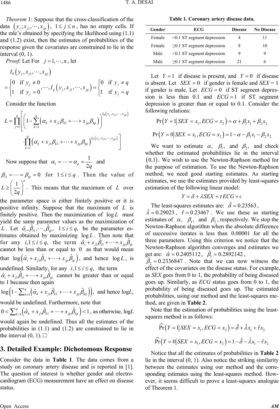 T. A. DESAI 1486 Theorem 1: Suppose that the cross-classification of the data 1 ;,, jj yx xp , , has no empty cells. If the mle’s obtained by specifying the likelihood using (1.1) and (1.2) exist, then the estimates of probabilities of the response given the covariates are constrained to lie in the interval (0, 1). 1jn Proof: Let For , let 1, ,jn 01 1 ,,, 0if 00if ,,,,, 1if 01if jj jp j qjj jp j Iyx x y Iyxx yy j j q q y Consider the function 01 1 ,,, 11 1 1 ,,, 11 1 1 jjp kjj jp Iyx x q n kjk jpkp k j qIyx x kjkjpkp k Lxx xx Now suppose that 1 1 2 qq and 10 iip for 1. Then the value of iq 1. 2 n Lq L This means that the maximum of over the parameter space is either finitely positive or it is positive infinity. Suppose that the maximum of is finitely positive. Then the maximization of must yield the same parameter values as the maximization of . Let 1ii ip L log L Lˆˆ ˆ,, ,, ,1 ,ii q be the parameter es- timates obtained by maximizing . Then note that for any the term 11i jpip 1iq, ˆ log L ˆij ˆ xx cannot be less than or equal to as that would mean 0 that 11 ˆˆ ˆ log iji jpip xx , and hence , is log L undefined. Similarly, for any the term 11 p ,1 ,iiq ˆ ˆiji jpi xx ˆ cannot be greater than or equal to 1 because then again 11 1 ˆ ˆ log 1, q kjkjpkp kxx ˆ 1 and hence logL, would be undefined. Furthermore, note that 11 1 ˆˆ ˆ 0 q kjkjpkp kxx , as otherwise, logL would again be undefined. Thus all the estimates of the probabilities in (1.1) and (1.2) are constrained to lie in the interval (0, 1). 3. Detailed Example: Dichotomous Response Consider the data in Table 1. The data comes from a study on coronary artery disease and is reported in [1]. The question of interest is whether gender and electro- cardiogram (ECG) measurement have an effect on disease status. Table 1. Coronary artery disease data. Gender ECG Disease No Disease Female <0.1 ST segment depression 4 11 Female ≥0.1 ST segment depression 8 10 Male <0.1 ST segment depression 9 9 Male ≥0.1 ST segment depression 21 6 Let 1Y if disease is present, and if disease is absent. Let 0Y 0SEX if gender is female and SEX = 1 if gender is male. Let if ST segment depres- sion is less than 0.1 and if ST segment depression is greater than or equal to 0.1. Consider the following relations: 0ECG EC 1 G 1211 Pr 1,YSEXxECGxxx 22 12 11 Pr 0,1YSEXxECGx x 22 x We want to estimate , 1, and 2, and check whether the estimated probabilities lie in the interval 0,1 . We wish to use the Newton-Raphson method for the purpose of estimation. To use the Newton-Raphson method, we need good starting estimates. As starting estimates, we use the estimates provided by least-squares estimation of the following linear model: YSEXECG The least-squares estimates are: , , ˆ0.23563 ˆ0.29023 ˆ0.23467 . We use these as starting estimates of , 1, and 2 , respectively. We stop the Newton-Raphson algorithm when the absolute difference of successive iterates is less than for all the three parameters. Using this criterion we notice that the Newton-Raphson algorithm converges and estimates we get are: 0.00001 ˆ0.2405112 , 1, 2. Note that we can now witness the effect of the covariates on the disease status. For example, as SEX goes from 0 to 1, the probability of being diseased goes up. Similarly, as ECG status goes from 0 to 1, the probability of being diseased goes up. The estimated probabilities, using our method and the least-squares me- thod, are given in Table 2. ˆ 0.2892142 ˆ0.2336 847 Note that the estimation of probabilities using the least- squares method is as follows: 121 ˆˆˆ Pr 1,YSEXxECGxxx 2 12 1 ˆˆˆ Pr 0,1YSEXxECGx xx 2 Notice that all the estimates of probabilities in Table 2 lie in the interval (0, 1). Also notice the striking similarity between the estimates using our method and the corre- sponding estimates using the least-squares method. How- ever, it seems difficult to prove a least-squares analogue of Theorem 1. Open Access AM 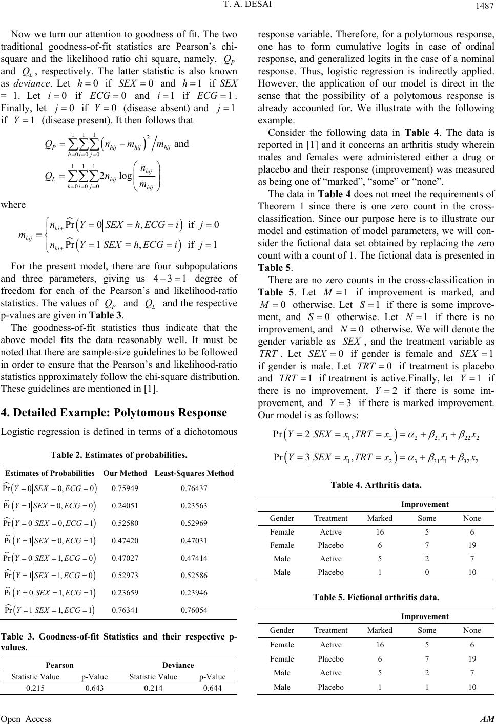 T. A. DESAI 1487 Now we turn our attention to goodness of fit. The two traditional goodness-of-fit statistics are Pearson’s chi- square and the likelihood ratio chi square, namely, Q and Q, respectively. The latter statistic is also known as deviance. Let if and if SEX = 1. Let if and if 0h ECG 0SEX 0 1h EC0i1i1G . Finally, let if Y (disease absent) and 0j01j if (disease present). It then follows that 1Y 111 2 00 0 111 00 0 and 2log Phij hijhij hi j hij Lhij hi jhij Qnmm n Qn m where Pr0,if 0 Pr1= ,if1 hi hij hi nYSEXhECGij m nYSEXhECGij resporiable. T, for aous rse, the following data in Table 4. The data is re irements of Th re no zero counts in the cross-classification in T For the present model, there are four subpopulations and three parameters, giving us degree of freedom for each of the Pearson’s and likelihood-ratio statistics. The values of 431 Q and Q and the respective p-values are given in Table 3. The goodness-of-fit statistics thus indicate that the above model fits the data reasonably well. It must be noted that there are sample-size guidelines to be followed in order to ensure that the Pearson’s and likelihood-ratio statistics approximately follow the chi-square distribution. These guidelines are mentioned in [1]. 4. Detailed Example: P ol yto mo us Res po nse Logistic regression is defined in terms of a dichotomous Table 2. Estimates of probabilities. Estimates of Probabilities Our Method Least-Squares Method Pr 00,0YSEX ECG 0.75949 0.76437 Pr 10,0Y SEXECG 0.24051 0.23563 Pr 00,1Y SEXECG 0.52580 0.52969 Pr 10,1Y SEXECG 0.47420 0.47031 Pr 01,0Y SEX ECG 0.47027 0.47414 Pr 11,0Y SEXECG 0.52973 0.52586 Pr 01,1YSEXECG 0.23659 0.23946 Pr 11,1Y SEXECG 0.76341 0.76054 Table 3. Goodness-of-fit Statistics and their respective p- values. Pearson Deviance Statistic Value p-Value Statistic Value p-Value nse vaherefore polytomespon one has to form cumulative logits in case of ordinal response, and generalized logits in the case of a nominal response. Thus, logistic regression is indirectly applied. However, the application of our model is direct in the sense that the possibility of a polytomous response is already accounted for. We illustrate with the following example. Consider ported in [1] and it concerns an arthritis study wherein males and females were administered either a drug or placebo and their response (improvement) was measured as being one of “marked”, “some” or “none”. The data in Table 4 does not meet the requ eorem 1 since there is one zero count in the cross- classification. Since our purpose here is to illustrate our model and estimation of model parameters, we will con- sider the fictional data set obtained by replacing the zero count with a count of 1. The fictional data is presented in Table 5. There a able 5. Let 1 if improvement is marked, and 0M otherwise.t 1S Le if there is some improve- and 0S ment, otherwise. Let 1N if there is no improvement, and 0N otherwis will denote the gender variable as , and the treatment variable as TRT . Let 0SEX e. We SEX if gender is female and 1SEX et 0TRT if treatment is placebo and 1TRT if gender is male. L if treatmeive.Finally, let 1Ynt is act if theremprovement, 2Y if there is som- provement, and 3Y is no ime i if th marked improvement. Our model is as follows: ere is 122211222 xx x Pr 2,YSEXx TRT 123311 Pr 3,YSEXxTRTxxx 322 Table 4. Arthritis data. ent Improvem Gender TreatmentMarked None Some Female Active 16 5 6 Female Placebo 6 7 19 Male Active 5 2 7 Male Placebo 1 0 10 Table 5. Fiction. al arthritis data Improvement Gender TreatmentMarked None 0.215 0.643 0.214 0.644 Some Female Active 16 5 6 Female Placebo 6 7 19 Male Active 5 2 7 Male Placebo 1 1 10 Open Access AM 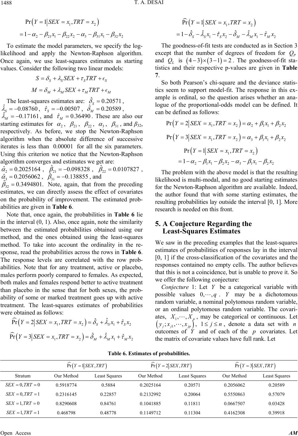 T. A. DESAI Open Access AM 1488 12 2211222331 1322 Pr 12 12 1 Pr 1, ˆˆ ˆˆ ˆˆ 1SS SMMM YSEXxTRTx 1SE ,TRT 1 YX xx xxx To estimate the model parameters, we specify the log- lik 2 xx x The goodness-of-fit tests are conducted as in Section 3 except that the number of degrees of freedom for Q and Q is 4331 2 . The goodness-of-fit sta- tistics and their respective p-values are given in Table 7. elihood and apply the Newton-Raphson algorithm. Once again, we use least-squares estimates as starting values. Consider the following two linear models: SSSS SSEXTRT So both Pearson’s chi-square and the deviance statis- tics seem to support model-fit. The response in this ex- ample is ordinal, so the question arises whether an ana- logue of the proportional-odds model can be defined. It can be defined as follows: MM MSEXTRT M ˆ The least-squares estimates are: , 0.20571 S ˆ 0.08760 S , ˆ0.00507 S , , , ˆ0.20589 M 0 ˆ0.17161 M and ˆ0.3649 M 2 . These are also s for our starting estimate , 21 , 22 , 3 , 31 , and β32, respectively. As befotoe w-Raphson algorithm when the absolute difference of successive iterates is less than 0.00001 for all the six parameters. Using this criterion we e that the Newton-Raphson algorithm converges and estimates we get are: 2 ˆ0.2025164 re, we s notic p thNeton , 21 ˆ0.098328 , 22 ˆ0.0 107827 12211 Pr 2,YSEXxTRTxx x 22 12311 Pr 3,YSEXxTRTxx x 22 12 211223112 Pr 1, 1 YSEXxTRTx 2 xxx , 3 ˆ0.2056062 32 ˆ0.349480 estimates, we ca , ˆ . t from the directly assess the effect of covariates on the probability of improvement. The estimated prob- abilities are given in Table 6. Note that, once again, the p 31 0.13885 Note, again, t n 5, and a 1hpreceding The problem with the above model is that the resulting likelihood is multi-modal, and no good starting estimates for the Newton-Raphson algorithm are available. Indeed, the author found that with some starting estimates, the resulting probabilities lay outside the interval [0, 1]. More research is needed on this front. robabilities in Table 6 lie in the interval (0, 1). Also, once again, note the similarity between the estimated probabilities obtained using our method, and the ones obtained using the least-squares method. To take into account the ordinality in the re- sponse, read the probabilities across the rows in Table 6. The response levels are correlated with the row prob- abilities. Note that for any treatment, active or placebo, males perform poorly compared to females. As expected, both males and females respond better to active treatment than placebo in the sense that for both sexes, the prob- ability of some or marked treatment goes up with active treatment. The least-squares estimates of probabilities were obtained as follows: 5. A Conjecture Regarding the Least-Squares Estimates We saw in the preceding examples that the least-squares estimates of probabilities of responses lay in the interval [0, 1] if the cross-classification of the covariates and the responses contained no empty cells. The author believes that this is not a coincidence, but is unable to prove it. So we offer the following conjecture: 12 Pr 2 ,YSEXxTRT 12 ˆˆˆ SS S xxx 12 1 ˆˆˆ Pr 3,MMM YSEXx TRTxxx 2 Conjecture 1: Let Y be a categorical variable with possible values . may be a dichotomous random variable, a nominal polytomous random variable, or an ordinal polytomous random variable. The covari- ates, 0,,q Y 1,, X, may be categorical or continuous. Let 1 ;,, jjp , yxx1jn , denote a data set with outcomes of Y and of each of the covariates. Let the matrix of covariate values have full rank. Let n p Table 6. Estimates of probabilities. Pr 1,YSEXTRT Pr 2,YSEXTRT Pr 3,YSEXTRT Strm Our Method Least Squares Our Method Least Squares Our Method Least Squares atu 0,TRT0SEX 0.5918774 0.5884 0.2025164 0.20571 0.2056062 0.20589 0, 1SEX TRT 0.2316145 0.22857 0.2132992 0.20064 0.5550863 0.57079 1, 0SEX TRT 0.8290608 0.84761 0.1041885 0.11811 0.0667507 0.03428 1, 1SEX TRT 0.468798 0.48778 0.1149712 0.11304 0.4162308 0.39918 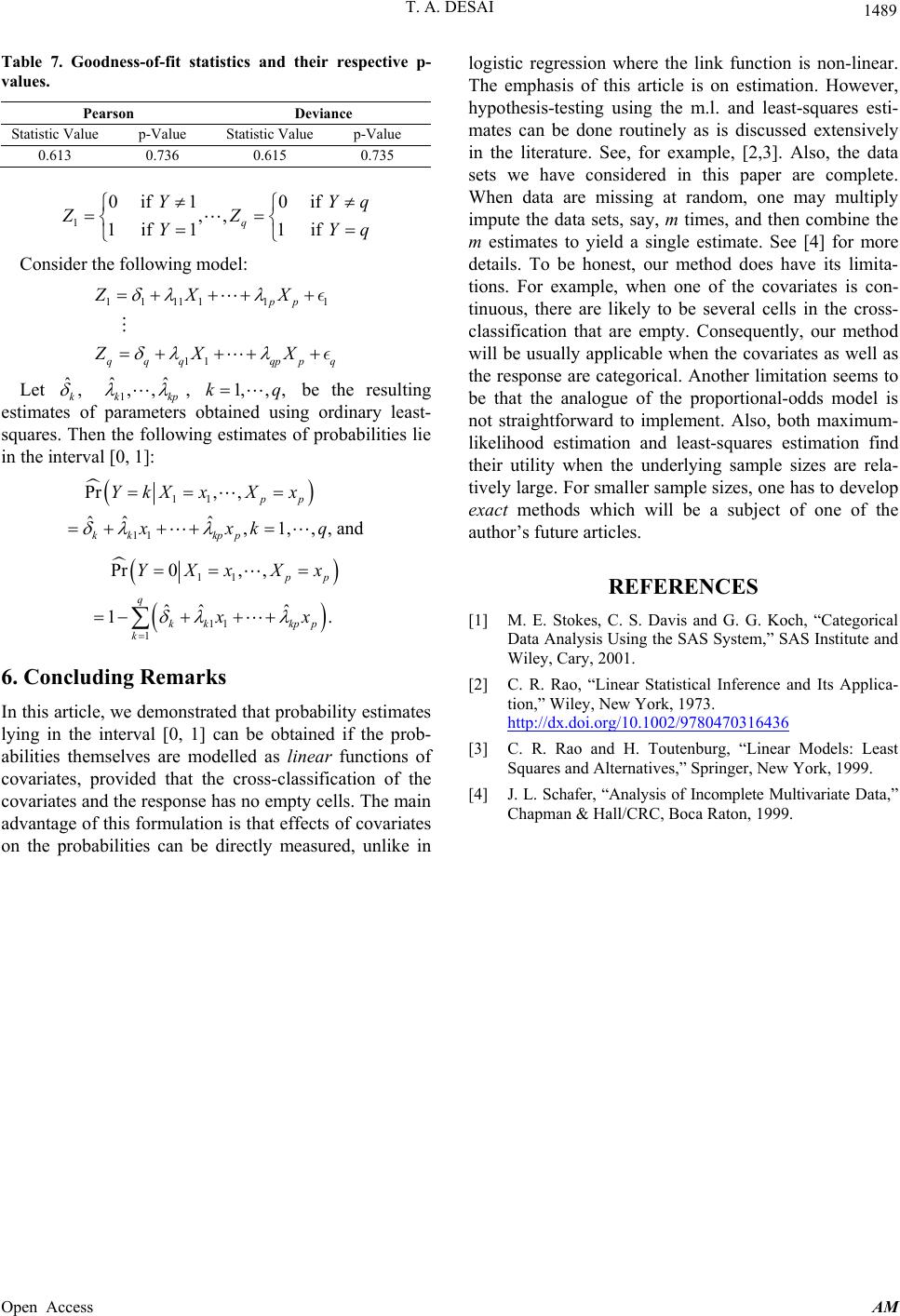 T. A. DESAI 1489 Table 7. Goodness-of-fit statistics and their respective p alues. - v Pearson Deviance Statistic Value p-Value Statistic Value p-Value 0.613 0.736 0.615 0.735 Y Yq Consider the following model: q Let 1 0i 1if ,, 1if11if q ZZ Y fY0q 11111 1 ZX 1 11 pp qqq qpp X ZXX ˆ, k 1 ˆˆ ,, kkp aramete , be the resulting est 1,, ,kq rs obtained usiimang ordinary least- squares. Then the following estimates of probabilities lie in the interval [0, 1]: tes of p Pr YkX 11 11 , , ˆˆ ˆ,1,,, and pp kk kpp xX x xxkq 11 11 1 Pr0, , ˆˆ ˆ 1. p q kk kpp k YXxXx xx 6. Concluding Remarks that probability esti stic regwhere thion isear. REFERENCES [1] M. E. Stokes,Koch, “Categorical Data Analysis Using th” SAS Institute and ork, 1973. In this article, we demonstratedmates lying in the interval [0, 1] can be obtained if the prob- abilities themselves are modelled as linear functions of covariates, provided that the cross-classification of the covariates and the response has no empty cells. The main advantage of this formulation is that effects of covariates on the probabilities can be directly measured, unlike in The emphasis of this article is on estimation. However, hypothesis-testing using the m.l. and least-squares esti- mates can be done routinely as is discussed extensively in the literature. See, for example, [2,3]. Also, the data sets we have considered in this paper are complete. When data are missing at random, one may multiply impute the data sets, say, m times, and then combine the m estimates to yield a single estimate. See [4] for more details. To be honest, our method does have its limita- tions. For example, when one of the covariates is con- tinuous, there are likely to be several cells in the cross- classification that are empty. Consequently, our method will be usually applicable when the covariates as well as the response are categorical. Another limitation seems to be that the analogue of the proportional-odds model is not straightforward to implement. Also, both maximum- likelihood estimation and least-squares estimation find their utility when the underlying sample sizes are rela- tively large. For smaller sample sizes, one has to develop exact methods which will be a subject of one of the author’s future articles. logiression e link funct non-lin C. S. Davis and G. G. e SAS System, Wiley, Cary, 2001. [2] C. R. Rao, “Linear Statistical Inference and Its Applica- tion,” Wiley, New Y http://dx.doi.org/10.1002/9780470316436 [3] C. R. Rao and H. Toutenburg, “Linear Squares and Alternatives,” Springer, New Y Models: Least ork, 1999. [4] J. L. Schafer, “Analysis of Incomplete Multivariate Data,” Chapman & Hall/CRC, Boca Raton, 1999. Open Access AM
|