Modern Economy, 2013, 4, 712-722
Published Online November 2013 (http://www.scirp.org/journal/me)
http://dx.doi.org/10.4236/me.2013.411077
Open Access ME
A Study of Changes in Risk Appetite in the Stock Market
and the Housing Market before and after the Global
Financial Crisis in 2008 Using the vKOSPI
Jin Yong Yang1*, Sang-Heon Lee2
1Hankuk University of Foreign Studies, Seoul, South Korea
2Hanyang University, Seoul, South Korea
Received October 7, 2013; revised November 5, 2013; accepted November 15, 2013
Copyright © 2013 Jin Yong Yang, Sang-Heon Lee. This is an open access article distributed under the Creative Commons Attribution
License, which permits unrestricted use, distribution, and reproduction in any medium, provided the original work is properly cited.
ABSTRACT
This study analyzes the empirical relationship between the vKOSPI, which is the Korean VIX (implied volatility index),
and the housing market (rent1-to-house price ratio) based on monthly data from January 2003 to November 2012. The
data were divided into two parts before and after the global financial crisis in 2008 and were analyzed by using the Vec-
tor Autoregressive (VAR) Model. The research results show that the influence of vKOSPI on the housing market
changes from symmetric to asymmetric since the global financial crisis in 2008. Before the global crisis in 2008, the
influence of the vKOSPI on the house price index and rent index is almost the same, so the influence on the
rent-to-house price ratio is not statistically significant. However, since the global crisis in 2008, the influence of the
vKOSPI on the two prices has changed asymmetrically and the influence on the rent-to-house price ratio was statisti-
cally significant. Second, the influence of the vKOSPI fluctuation on house sale prices and rent is shown differently
according to the rise/fall of the vKOSPI. In the event of the vKOSPI rising, house prices would fall greatly. On the
other hand, in the event of the vKOSPI falling, the rise in housing prices is relatively small. This means that while the
boosted sentiment of investors in the stock market is not transferred to the housing sales market, the aggravated senti-
ment of investors affects the housing sales market easily. In conclusion, the uncertainty has been represented in the
vKOSPI and the preference for risky assets has an asymmetrical influence on the market dependent upon the kind of
market. We suspect that this is caused by complex factors including shrinking expectations for future house prices.
Keywords: Risk Appetite; Stock Market; Housing Market; Implied Volatility Index
1. Introduction
The major factors that influence the housing market are
economic circumstances (this is a fundamental factor),
economic bubbles, and policies. Since a house is a risky
asset, it is affected by the sentiment of investors. The
global financial crisis in the latter half of 2008 began in
the USA and spread worldwide. It originated from the
real estate crisis. It is widely recognized that rapid fluc-
tuation of real estate prices had a negative influence on
the economy. Most economic specialists suspect that low
interest rates and excessive mortgage loans created the
soaring house prices in the USA, and the fall of the col-
lateral value of a house due to the collapse of the housing
bubble generated inferior assets in the banks.
Rise of real estate prices stimulates economic activities
by the wealth effect and increases investment and con-
sumption expenditures. This also indirectly increases the
demands for loans. The rise of real estate prices increases
the collateral value of the borrowers. This is called the
financial accelerator effect (Bernanke et al. [1]).
In particular, from 2009 to 2012, the rise of rent is
greater than the rise of house sale prices in the Korean
housing market, most of which is interpreted as due to
the changes in the sentiment of investors. Notwithstand-
ing, there is no specific problem in housing supply, peo-
ple have come to prefer renting compared to the purchase
of a house when choosing their residence. Therefore, it is
*Corresponding author.
1This means “Jeonse” price, deposit money for housing lease. “Jeonse”
is a unique system of Korea. A lessee deposits a certain amount of mo-
ney to the owner during the lease period and gets back the full amount
of the money at the end of leasing.

J. Y. YANG, S.-H. LEE 713
interpreted that the sentiment of investors toward the
housing market has changed.
According to a news article2, rental prices have con-
tinuously risen since the global financial crisis and there
have been an increasing number of loans given for pro-
viding a rental deposit. In particular, due to the rise of
rentals, the total market price of rentals nationwide
reaches almost half of the total market price of house
sales. The key point of the article is that there is a lot of
demand for rental properties, but consumers are not
shifting to the sales market. This is because investors be-
lieve that paying a rental deposit is better than buying a
house which has a larger debt burden.
The vKOSPI is a volatility index that represents the
future outlook of investors who participate in stock mar-
ket. It is also referred to as the “fear index”.
In the USA, the VIX, an index to represent volatility
of the stock market, is used as an overall measure that
shows uncertainty (e.g. Bloom [2]). The Korean Volatil-
ity Index, vKOSPI, also represents the degree of uncer-
tainty that Korean investors feel at a given moment. Ac-
cording to Chauvet, Gabriel and Lutz [3], VIX, the index
representing the attitude of investors who participate in
the stock market with a focus on risk, and the Housing
Distress Index (HDI) from the housing market demon-
strate a very similar pattern. Therefore, the vKOSPI also
may be considered to be connected with the psychologi-
cal flow of investors.
This study analyzes the influence of the attitude or risk
appetite of investors towards risky assets, which is rep-
resented as the KOSPI Volatility Index (vKOSPI), on the
housing market.
The distinctive features of this study compared to pre-
vious studies are outlined below.
First, this study investigates the relationship between
the vKOSPI and the housing market, unlike other studies
that analyze the relationship between the housing sales
market and rental market. Few studies have been con-
ducted in that way so far.
Second, using the house price to rent ratio, it aims to
have consistency with the index that is mainly used by
market participants.
Third, it analyzes the influence of the vKOSPI on the
housing market before and after the global financial cri-
sis in 2008 using the VAR model.
Major research results are explained below.
First, the influence of the vKOSPI on the housing
market before and after the global financial crisis in 2008
changed from symmetric to asymmetric. Before the eco-
nomic crisis in 2008, the influences of the vKOSPI on
the house price index and rent index are very similar to
each other, symmetrically that is, the influence on the
rent-to-house price ratio is not statistically significant. It
is because the vKOSPI has a similar influence on both
the denominator and numerator of the rent-to-house price
ratio. However, after the economic crisis in 2008, the
effect of the vKOSPI is asymmetric, which is statistically
significant.
Second, the vKOSPI has a bigger influence on the rent
index than the house price index. This is a very interest-
ing point. To explain in more detail, when the vKOSPI
falls, both rent and house prices rise. However, the rise in
rent prices is larger than the rise in house prices, which
makes the changes in rent-to-house price ratio bigger.
On the other hand, when the the vKOSPI rises, both
rent and house prices fall. In that case, the fall in house
prices is larger than the fall in rents, which makes the
changes in rent-to-house price ratio smaller. This means
that the vKOSPI fluctuation had different influences on
house prices and rent according to the rise/fall of the
vKOSPI. Although the sentiment of participants in the
stock market is boosted due to the fall of the vKOSPI,
the prices in the rental market rise more than the housing
market. It means that the boosted sentiment of investors
in the stock market does not often shift to the housing
market. It also means that although the sentiment of par-
ticipants in the stock market is aggravated due to the rise
of the vKOSPI, the fall of house prices is much bigger
than the rental market, causing the stock market to easily
affect the housing market. 1) When the risk appetite of
investors changes in regard to the uncertainty and risk
due to the vKOSPI fluctuation, the volatility increases in
the rental market more than in the house sales market;
and 2) the asymmetric sentiment of investors is trans-
ferred from the stock market to the housing market.
These results show that investors have a different attitude
towards participating in the two markets.
Third, when the vKOSPI rises, the changes in rent-to-
house price ratio increase more than the case when the
vKOSPI falls (asymmetric effect). This coincides with a
general phenomenon in which the volatility gets bigger
when stock prices fall, than the case when stock prices
rise. The direction of volatility and the price variable of
the housing market show similar patterns.
Last, the vKOSPI “Granger causes” the changes in rent-
to-house price ratio. This means that the risk attitude of
investors who participate, based on uncertainty in stock
market, is closely related to the price variable of the hous-
ing market.
The structure of the research is as follows. Chapter 2
summarizes previous studies and Chapter 3 summarizes
the data. Chapter 4 provides methodology and Chapter 5
presents the results. Chapter 6 offers some conclusions.
2News article from the internet, “The rent soared up... scarcity for rental
“Concerning on rental shortage”, http://news.naver.com/main/read.nhn?
mode=LSD&mid=sec&sid1=101&oid=001&aid=0006356773
Open Access ME

J. Y. YANG, S.-H. LEE 714
2. Previous Studies
Most previous studies focus on the relationship between
the stock market and housing market. They deal with the
issues concerning whether the two markets are co-inte-
grated or if there is any causality between the two mar-
kets. Apergis and Lambrinid is [4] show that the stock
market and the real estate market move together toward
the same direction (integration of the stock market and
real estate market) in the USA and UK by using co-inte-
gration and the error correction model with data from
1986 to 2006. They argue that as the integration of two
markets is great, a portfolio that contains both stocks and
real estate assets have relatively small advantages.
Anoruo and Braha [5] use the GARCH-enhanced
VECM model and focus on the rate of returns of the
houses and stocks. They insist that there is a co-integra-
tion relationship between the two factors. There is a
spillover effect from the stock market to the housing
market but the spillover effect doesn’t occur in the oppo-
site direction.
Sim and Chang [6] find that there is Granger causality
from house and land prices to stock prices, but doesn’t
find Granger causality in the opposite direction.
Tse [7] analyzes the relationship between the stock
market and real estate market by using Hong Kong data
from 1974 to 1998. As a result, he finds that unexpected
change in real estate prices is a main factor that can in-
fluence stock prices and that the two markets are co-in-
tegrated. As a high portion of real estate-related compa-
nies are listed on the stock market, the trend of real estate
prices affects the profitability of the real estate-related
companies, which in turn has an influence on their stock
prices.
Unlike previous studies, this study analyzes the effect
of the vKOSPI on the housing market, and also the effect
of the investors’ attitude toward risk in the housing mar-
ket. As there are various influential factors that affect the
housing market, this study use macroeconomic variables
as additional explanatory variables, in order to control
the effect.
3. Data
3.1. Relationship between the VIX and the
Housing Market Index
Figure 1 is a graph shown in the paper of Chauvet,
Gabriel and Lutz [3] to compare the HDI and VIX. The
dotted line represents the VIX, and the solid line the HDI.
As shown in Figure 1, the sentiments of investors who
participate in the two markets have differences in volatil-
ity but very similar patterns in terms of trend.
3.2. Basic Data
The data used in model estimation is the house price in-
Figure 1. VIX and HDI.
dex, rent index, KOSPI index, consumer price index,
index of industrial production, vKOSPI index and esti-
mated data series related to term structure of interest
rates. The data related to term structure of interest rates
refers to the level and slope factors estimated by the Dy-
namic Nelson Siegel model (hereafter DNS model) on
the spot yield curve of government bonds. The estimated
level and slope factor are used instead of the interest
rates of government bonds with a specific maturity. This
is because of the fact that the term structure of govern-
ment bonds can be represented in the three factors of le-
vel, slope, and curvature3.
The data is collected on a monthly basis and the sam-
pling period is from January 2003 to November 2012.4
The time series of basic data are shown in Figure 2.
Analyzing the data before and after the global finan-
cial crisis triggered by the bankruptcy of Lehman Broth-
ers Holdings in the 3rd quarter of 2008 (hereinafter re-
ferred to as the global financial crisis in 2008), we can
find a few characteristics. First, the rent-to-house price
ratio of a house is falling until the global financial crisis
in 2008, but after the crisis until 2012 it rises. Second,
the level of the yield curve since the global financial cri-
sis in 2008 lowers gradually due to expansionary mone-
tary policy in reaction to the crisis, and the term structure
of interest rates make a parallel shift downwards. The
slope of the yield curve increases dramatically and then
gradually decreases over time, eventually returning to a
value close to the long-term average.5 Table 1 shows the
basic statistics of transformed data.
The results found through the analysis of the correla-
tion of Table 1 can be summarized as follows.
First, as for the rent-to-house price ratio, the housing
3The relationship between the three factors of the term structure o
f
interest rates and economic variables is explained in detail in the re-
search of Diebold et al. [8].
4The starting point of the vKOSPI data is January 2003.
5The figures of the slope factor in the DNS model are the values of the
normal slope to which all, minus (−) was prefixed. Therefore, as the
value of the slope factor decreases, the slope of the actual term of the
structure increases. See Diebold et al. [8].
Open Access ME

J. Y. YANG, S.-H. LEE
Open Access ME
715
60
70
80
90
100
110
02 03 04 05 06 07 08 09 10 1112
HOUSE
70
80
90
100
110
02 03 04 05 06 07 08 09 10 1112
JEONS E
0.90
0.95
1.00
1.05
1.10
1.15
02 03 04 05 06 07 08 09 101112
JP_ HP
400
800
1,200
1,600
2
,000
2
,400
02 03 04 05 06 07 08 09 10 1112
KOSPI
.0
.2
.4
.6
.8
02 03 04 05 06 07 08 09 10 1112
VKOSPI
70
80
90
100
110
02 03 04 05 06 07 08 09 101112
CP I
50
60
70
80
90
100
110
02 03 04 05 06 07 08 09 10 1112
IP
.03
.04
.05
.06
.07
.08
02 03 04 05 06 07 08 09 10 1112
DNS_ALPHA
-.05
-.04
-.03
-.02
-.01
.00
02 03 04 05 06 07 08 09 101112
DNS _B ETA
2011.06=100
2010=100
dec im al
dec im al
dec im al
2010=100
2011.06=100
1980.1.4=100
0.8
0.6
0.4
0.2
0.0
0.08
0.07
0.06
0.05
0.04
0.03
0.00
−0.01
−0.02
−0.03
−0.04
−0.05
2400
2000
1600
1200
Figure 2. Basic data. *HOUSE: house price index; JEONSE: rent index; JP_HP: rent-to-house price ratio; KOSPI: KOSPI
index; vKOSPI: KOSPI 200 volatility index; CPI: consumer price index; IP: index of industrial production; DNS_ALPHA:
level factor, and DNS_BETA: slope factor. *The units of basic data for this study are used asis. vKOSPI, DNS_ALPHA and
DNS_BETA, were not multiplied by 100. Therefore, these three sets of data should be read in decimal not in percentage (%).
market has changed since the global financial crisis in
2008. The rent-to-house price ratio and house prices have
a negative (−) correlation between the Pre-crisis period
(the period before the crisis) and the Entire period (the
whole period of the data covering before and after the
crisis). It means that the bigger the changes in the
rent-to-house price ratio are, the lower the house prices
are. On the contrary, the bigger the changes in house
prices are, the smaller the changes in rent-to-house price
ratio are. It is because the rise of house prices is bigger
than the rise of rents. However, after the global financial
crisis in 2008, the correlation between the rent-to-house
price ratio and house prices is shown as positive (+). It
means that after the global financial crisis in 2008, the
higher the changes in rent-to-house price ratio, the higher
the rise in house prices. Although it may be an unex-
pected result, the correlation between rent-to-house price
ratio and rent can justify the result. The correlation be-
tween rent-to-house price ratio and rent during the
Post-crisis period is 0.857, which shows that the rise of
rents is relatively higher than the rise of house prices.
Therefore, from the perspective of market participants, it
shows that rents rise higher than house prices do.
Second, the relationship between the stock market and
housing market vary according to the attitude of inves-
tors towards the markets’ direction and risk. The KOSPI
index shows positive (+) correlation with house prices,
but negative (−) with rental prices. On the other hand, the
vKOSPI have a positive (+) relationship with both house
and rental prices. It means that whereas the direction of
the stock market is correlated with house prices and rent-
als in opposite directions, the sentiment of investors on

J. Y. YANG, S.-H. LEE 716
Table 1. Correlation of the data among pre-crisis, post-crisis, and the entire period of the financial crisis in 2008.
sample HOUSE JEONSE JP_HP KOSPI ALPHA BETA CPI IP
Pre-crisis 0.639
Post-crisis 0.919 JEONSE
Entire 0.576
Pre-crisis −0.582 0.253
Post-crisis 0.576 0.851 JP_HP
Entire −0.405 0.513
Pre-crisis 0.017 −0.128 −0.167
Post-crisis 0.014 −0.014 −0.052 KOSPI
Entire 0.026 −0.089 −0.135
Pre-crisis −0.051 0.200 0.271 −0.319
Post-crisis 0.011 −0.102 −0.272 0.063 ALPHA
Entire 0.055 −0.116 −0.199 −0.040
Pre-crisis 0.239 0.188 −0.098 0.057 −0.323
Post-crisis −0.145 −0.108 0.014 −0.325 −0.730 BETA
Entire 0.129 −0.172 −0.311 −0.130 −0.353
Pre-crisis −0.171 0.117 0.344 −0.167 0.231 0.011
Post-crisis 0.135 0.099 0.017 0.139 0.142 −0.257 CPI
Entire −0.069 0.073 0.156 −0.035 0.179 −0.072
Pre-crisis −0.112 0.042 0.179 0.080 −0.054 0.009 0.010
Post-crisis 0.259 0.246 0.156 0.197 −0.050 −0.423 0.256
IP
Entire 0.025 0.128 0.110 0.142 −0.035 −0.228 0.121
Pre-crisis −0.206 −0.247 −0.020 −0.264 0.339 0.081 0.053 −0.076
Post-crisis −0.481 −0.536 −0.472 −0.287 0.320 0.117 −0.193 −0.372 VKOSPI
Entire −0.289 −0.349 −0.091 −0.270 0.265 0.044 −0.087 −0.270
*Pre-crisis: From January 2003 to August 2008; Post-crisis: From September 2008 to November 2012, and Entire period: From January 2003 to November 2012.
*House prices, rents, KOSPI index, index of industrial production, and consumer price index were log differentiated. Rent-to-house price ratio was differenti-
ated. The level variables were used as they were for level factor, slope factor, and the vKOSPI.
implied volatility or risk in the stock market have a nega-
tive (−) relationship with the two markets.
Third, the correlations of vKOSPI with rents, and
house prices show a big difference from the correlation
between the vKOSPI and the rent-to-house price ratio.
The correlations of vKOSPI with rents, and house prices
are negative (−), regardless of the global financial crisis
in 2008. One thing that is noteworthy is that the correla-
tion after the crisis in 2008 becomes greater. The rela-
tionship between the vKOSPI and the rent-to-house price
ratio is also negative (−), but it becomes much greater
(−0.02  −0.472) after the crisis in 2008. Before the
crisis in 2008, the vKOSPI affect a similar amount of
house prices and rents, which is a symmetric influence.
However, after the crisis, it has influence of a different
size, that is, an asymmetric influence. In other words,
before the crisis in 2008, when both the stock market and
housing market are on the rise, the attitude of investors
participating in the housing sales market and rental mar-
ket toward risky assets shows a similar pattern. After the
crisis in 2008, however, there is a remarkable difference
in the attitude of the investors in the sales market and
rental market. It is assumed that the uncertainty in ex-
pected rising house prices have influence on the inves-
tors’ appetite for houses, a risky asset.
Fourth, it is noteworthy that the correlation between
the vKOSPI and housing market (sales and rental) after
the global financial crisis in 2008 is bigger than the cor-
relation between the vKOSPI and stock market. In par-
ticular, the correlation between the vKOSPI and rental/
house prices index before and after the global financial
crisis in 2008 is −0.02, and −0.472, respectively, which is
a significant increase.
Fifth, the industrial production index and consumer
price index that represent the basic conditions of the
economy over the Entire period show positive (+), and
negative (−) relationships with the house prices, respec-
tively.
Open Access ME

J. Y. YANG, S.-H. LEE 717
4. Methodology
Before conducting the analysis on the relationship among
the stock market, housing market, and economic vari-
ables, unit root and co-integration tests are conducted.
The model that is most suitable for the changes before
and after the global financial crisis in 2008 is the VAR
model.
4.1. Unit Root Test
All level variables of basic data have a unit root. There-
fore, unit root tests are conducted only on the converted
variables and all the results are stationary as shown in
Table 2. In particular, the rent index has a unit root even
when conducting the first order difference. It becomes
stationary after conducting the second order difference.6
In the event that the rent-to-house price ratio is used
without separating the house prices from rents, stationar-
ity is secured through the first order difference, regard-
less of setting the unit root test. Although the level and
slope factor in DNS model has a unit root, when esti-
mating DNS term structure model, data transformation is
not conducted because it is estimated on the assumption
that the level and slope factors follow stationary AR(1)
processes, respectively. Table 2 shows the results of the
unit root test on the variables that form the model.
By rejecting the null hypothesis of the Augmented
Dicky-Fuller Test (ADF), insisting that all variables ex-
cept for level and slope factors have a unit root at the
significant level of 5%, we find that the variables are
converted to stationary variables.
4.2. Co-Integration Test
If all variables have a unit root in I(1), first order differ-
encing makes them stationary time series. However, in
case of using first order differenced variables, there is a
risk of losing the information about the long-run rela-
tionships. The linear or non-linear relationship among dif-
ference variables cannot be interpreted as a long-run
equilibrium relationship.
In order to find out if a long-term equilibrium rela-
tionship exists in the stock market and housing market, a
co-integration test is conducted on the KOSPI index and
rent-to-house price ratio by log. Tables 3 and 4 show the
results with the use of Trace statistics and Max statistics.
As a result of the co-integration test, it is found that
there is no consistent co-integration relationship between
the KOSPI and rent-to-house price ratio, but a slight rela-
tion is found after the global financial crisis in 2008. As
for the co-integration relationship between the KOSPI
Table 2. Results of unit root test on the transformed vari-
ables.
t-value Prob.
DL_HOUSE −4.53471 0.0000
DL_JEONSE −2.07544 0.0369
D_JP_HP −2.56690 0.0105
DL_KOSPI −10.5752 0.0000
DNS_ALPHA −1.33450 0.1678
DNS_BETA −1.18927 0.2134
DL_CPI −8.68155 0.0000
DL_IP −9.80998 0.0000
*The meaning of the prefix affixed to the name of variables is as follows:
DL: log difference, D: difference.
Table 3. Co-integration test results using trace statistics.
Sample periodNo. of
CE(s) Eigenvalue Statistic Critical Value Prob.
None 0.112362 11.27182 15.494710.1953
Pre-crisis At most 10.045503 3.166829 3.8414660.0751
None 0.24687 14.46376 15.494710.0711
Post-crisis At most 18.51E-05 0.004342 3.8414660.9462
None 0.093027 12.062 15.494710.154
Entire periodAt most 10.003712 0.442495 3.8414660.5059
*Pre-crisis: From January 2003 to August 2008, Post-crisis: From September
2008 to November 2012, and Entire period: From January 2003 to Novem-
ber 2012.
Table 4. Co-integration test results using Max statistics.
Sample periodNo. of
CE(s) Eigenvalue Statistic Critical Value Prob.
None 0.112362 8.104995 14.26460.3681
Pre-crisis At most 10.045503 3.166829 3.8414660.0751
None 0.24687 14.45942 14.26460.0466
Post-crisis At most 18.51E-05 0.004342 3.8414660.9462
None 0.093027 11.61951 14.26460.1258
Entire periodAt most 10.003712 0.442495 3.8414660.5059
*Pre-crisis: From January 2003 to August 2008, Post-crisis: From September
2008 to November 2012, and Entire period: From January 2003 to Novem-
ber 2012.
and rent-to-house price ratio, it doesn’t exist during the
Pre-crisis or the Entire period. After the crisis, however,
only Max statistics shows that a single co-integration re-
lationship existed while trace statistics shows no co-in-
tegration relationship. It can be interpreted that there is a
co-integration relationship between the stock market and
housing market after the crisis in 2008. Nonetheless,
since Max statistics and Trace statistics show different re-
sults, this study uses the VAR model which can be used
consistently to compare the Pre-crisis, Post-crisis, and En-
tire period.
6In case of conducting the unit root test, second order difference which
contains intercept, or trend and intercept gave a stationary value. I
f
none is included, the result becomes stationary only through the first
order difference.
Open Access ME

J. Y. YANG, S.-H. LEE
Open Access ME
718
5. Estimation Results 4.3. VAR Model
5.1. Estimation of the VAR Model
Representing the variables of the VAR model as column
vector t
X
, the VAR(1) model is formed as follows. Seeing the Tables 5-7, we can identify a few significant
exploratory variables before and after the global financial
crisis in 2008.

171
,~ 0,Σ
tttt
XABX N

  77
First, the changes in the vKOSPI level have a negative
(−) influence on the changes in rent-to-house price ratio
after the financial crisis in 2008. The results show the
same negative (−) correlation even on the data of the
Pre-crisis and Entire period and they are not statistically
significant. The vKOSPI may represent risk appetite of
investors in the stock market. That is, when the uncer-
tainty increases and the appetite of investors for risky
assets decreases proportionally by the rise of the vKOSPI,
both rent and house prices fall. In that case, rent (nu-
merator) falls less than house prices (denominator). On
the contrary, when the uncertainty decreases and the ap-
petite of investors for risky assets increases proportion-
ally by the fall of the vKOSPI, both rent and house prices
rise. In that case, the numerator, rent, rises much higher
than the denominator, house prices.




d logKOSPI
dJP HP
dlog IP
dlogCPI
vKOSPI
t
tt
t
tt
t
t
t
X













Here, dlog represents log difference and d represents
difference. The vector of time series variables, t
X
re-
presents KOSPI volatility, changes in rent (JP)-to-house
price (HP) ratio, level factor of interest rate, slope factor
of interest rate, growth rate of industrial production (IP),
inflation rate, and KOSPI 200 volatility index (vKOSPI),
in that order. “A” is a column vector of 7 × 1 constant
term; and “B” is 7 × 7 coefficient matrix. “t ” follows
multivariate normal distribution in which the average is
“0”and covariance is “Σ”.
Seeing the asymmetric changes in the rent-to-house
price ratio according to the changes in the vKOSPI, we
may suspect that when the investors’ appetite for the ris-
ky assets rises due to the fall of the vKOSPI, house pri-
ces will be more responsive than rents, but the actual data
shows the contrary. Rather, the result that the rise of
7177
The VAR model is estimated by using the OLS
method.
Table 5. VAR model estimation before the global financial crisis in 2008.
KOSPI JP_HP ALPHA BETA IP CPI VKOSPI
KOSPI(-1) −0.1291 0.0051 0.0013 −0.0049 0.0734 0.0007 0.0341
(−0.9615) (0.6269) (0.3110) (−0.9481) (1.6298) (0.0746) (0.4823)
JP_HP(-1) 0.1626 0.5817 0.0913 −0.0502 1.3950 0.0109 0.5456
(0.0912) (5.4218) (1.5845) (−0.7261) (2.3320) (0.0922) (0.5817)
ALPHA(-1) −6.4268 0.0404 0.8089 0.2373 −0.3138 0.0725 2.8184
(−2.3410) (0.2448) (9.1268) (2.2301) (−0.3409) (0.3984) (1.9528)
BETA(-1) −0.8693 −0.0075 0.0138 0.9545 0.0024 0.0792 0.3077
(−0.6222 (−0.0892) (0.3051) (17.6245) (0.0051) (0.8548) (0.4190)
IP(-1) 0.1966 −0.0160 −0.0053 −0.0031 −0.4426 −0.0303 0.0214
(0.5799) (−0.7861) (−0.4799) (−0.2339) (−3.8932) (−1.3483) (0.1201)
CPI(-1) −0.4646 0.2144 0.0044 −0.0604 0.4754 0.2355 −0.0936
(−0.2258) (1.7328) (0.0657) (−0.7577) (0.6892) (1.7254) (−0.0865)
VKOSPI(-1) 0.0819 −0.0122 −0.0059 0.0024 −0.0173 0.0016 0.7707
(0.5865) (−1.4521) (−1.3170) (0.4428) (−0.3692) (0.1682) (10.4948)
C 0.3322 −0.0010 0.0121 −0.0137 0.0307 −0.0012 −0.0928
(2.4543) (−0.1186) (2.7626) (−2.6013) (0.6774) (−0.1322) (−1.3038)
Adj. R-squared −0.0008 0.3993 0.6490 0.8386 0.1775 0.0022 0.6997
S.E. equation 0.0598 0.0036 0.0019 0.0023 0.0200 0.0040 0.0314
F-statistic 0.9926 7.2683 18.4322 49.9730 3.0341 1.0208 22.9685
*The figure in parentheses represents t-value.

J. Y. YANG, S.-H. LEE 719
Table 6. VAR model estimation after the global financial crisis in 2008.
KOSPI JP_HP ALPHA BETA IP CPI VKOSPI
KOSPI(-1) −0.1391 −0.0092 −0.0143 0.0032 0.0275 0.0055 −0.0898
(−0.9594) (−2.8630) (−2.4357) (0.3866) (0.4956) (0.7112) (−0.7605)
JP_HP(-1) −0.1973 0.4462 −0.0655 0.5161 −4.2910 −0.5061 3.0315
(−0.0504) (5.1468) (−0.4112) (2.2969) (−2.8607) (−2.4431) (0.9502)
ALPHA(-1) −7.2605 −0.0558 0.8795 0.1734 −2.6130 0.0169 8.4658
(−3.3490) (−1.1639) (9.9843) (1.3943) (−3.1484) (0.1476) (4.7955)
BETA(-1) −5.3201 −0.0271 −0.0816 1.0508 −1.7129 −0.0065 5.1329
(−4.0489 (−0.9319) (−1.5288) (13.9445) (−3.4054) (−0.0941) (4.7974)
IP(-1) −0.5354 −0.0013 0.0186 −0.0094 0.0282 0.0082 0.9265
(−1.3787 (−0.1466) (1.1763) (−0.4221) (0.1899) (0.3990) (2.9301)
CPI(-1) −0.9089 0.3039 −0.0712 0.0105 0.1040 0.2826 1.6292
(−0.3414) (5.1586) (−0.6580) (0.0689) (0.1020) (2.0079) (0.7515)
VKOSPI(-1) 0.1907 −0.0066 0.0028 −0.0145 −0.0373 −0.0056 0.7554
(2.1193) (−3.3224) (0.7758) (−2.8039) (−1.0821) (−1.1829) (10.3081)
C 0.2058 0.0050 0.0033 −0.0051 0.1183 0.0034 −0.2624
(2.3148) (2.5322) (0.9092) (−0.9949) (3.4773) (0.7168) (−3.6245)
Adj. R-squared 0.2012 0.7284 0.9028 0.9369 0.3867 0.1534 0.8439
S.E. equation 0.0591 0.0013 0.0024 0.0034 0.0226 0.0031 0.0481
F-statistic 2.7996 20.1600 67.3691 106.9870 5.5032 2.2939 39.6024
*The figure in parentheses represents t value.
Table 7. VAR model estimation during the Entire period (January 2003-November 2012).
KOSPI JP_HP ALPHA BETA IP CPI VKOSPI
KOSPI(-1) −0.0345 −0.0026 −0.0035 −0.0046 0.0761 0.0038 −0.0983
(−0.3478) (−0.5578) (−0.9661) (−0.9611) (2.0104) (0.6523) (−1.4066)
JP_HP(-1) −2.1752 0.6332 −0.0187 0.0756 −0.2686 −0.0779 1.7967
(−1.5043) (9.4225) (−0.3555) (1.0922) (−0.4874) (−0.9277) (1.7650)
ALPHA(-1) −1.9439 −0.1478 0.9726 0.1011 −0.4046 0.0407 2.3489
(−1.5876) (−2.5977) (21.7820) (1.7247) (−0.8672) (0.5717) (2.7248)
BETA(-1) −1.2720 −0.0865 0.0015 0.9898
−0.5088 −0.0056 1.1253
(−1.9980) (−2.9244) (0.0656) (32.4889) (−2.0974) (−0.1525) (2.5108)
IP(-1) 0.2043 −0.0151 0.0141 −0.0102 −0.0693 −0.0075 0.1256
(0.8293) (−1.3150) (1.5724) (−0.8622) (−0.7386) (−0.5262) (0.7241)
CPI(-1) −0.0329 0.2206 −0.0179 −0.0368 1.1648 0.3050 −0.5072
(−0.0200) (2.8833) (−0.2989) (−0.4666) (1.8568) (3.1890) (−0.4377)
VKOSPI(-1) 0.0696 −0.0042 −0.0011 −0.0125 −0.0437 −0.0016 0.8182
(0.9832) (−1.2701) (−0.4389) (−3.6974) (−1.6183) (−0.3922) (16.4169)
C 0.0728 0.0069 0.0015 −0.0020 0.0258 −0.0001 −0.0584
(1.2635) (2.5732) (0.7158) (−0.7189) (1.1745) (−0.0423) (−1.4413)
Adj. R-squared −0.0026 0.6223 0.8540 0.9301 0.1033 0.0511 0.7664
S.E. equation 0.0625 0.0029 0.0023 0.0030 0.0238 0.0036 0.0440
F-statistic 0.9575 28.5422 98.7818 223.3569 2.9248 1.8998 55.8412
*The figure in parentheses represents t-value.
Open Access ME

J. Y. YANG, S.-H. LEE
Open Access ME
720
house prices is smaller than the rise of rents shows that
the investors’ appetite for the risky assets, such as stocks,
does not totally shift to the housing sales market, in spite
of the rise of the investors’ appetite for the risky assets.
This means that the investors’ expectation for the hous-
ing market has changed and such a change is more ac-
celerated after the global financial crisis in 2008.
If the investors’ appetite for the risky assets falls due
to the rise of the vKOSPI, the fall in house prices gets
bigger than the fall in rents. It means that when the in-
vestors’ appetite for the risky assets, such as stocks de-
creases, their appetite for the risky assets is shifted to the
housing sales market.
The reasons for such an asymmetric influence of the
vKOSPI on the housing market may be considered from
various perspectives. From the perspective of the risk
appetite of investors, it is related to the situation where
the house price bubble collapses after the global financial
crisis and the expectation for the rise of house prices in
the future has not recovered yet.
Referring to the correlation analysis in Table 1, the
vKOSPI shows a negative (−) relationship with rents and
house prices. In terms of relative volatility after the fi-
nancial crisis in 2008, rents show more asymmetric
changes than house prices.
Second, the level factor of the government bond yield
curve (ALPHA) has a negative (−) influence on the stock
market, which shows the same pattern before and after
the financial crisis. During the Pre-crisis, if the term
structure moves upwards, the returns of the KOSPI fall
(−6.4268) and the level of vKOSPI rises. It is suspected
that due to the overall economic contraction triggered by
the rise of long-term and short-term interest rates, the rise
of stock market growth becomes sluggish and the risk
appetite of investors falls (rise of the vKOSPI). It shows
the same pattern after the crisis of 2008. The significance
of the estimated coefficient is higher and the size of the
coefficient is bigger, too. As shown in Table 7, when
estimation is made over the Entire period, the signifi-
cance falls, but the trend of the figures still remain nega-
tive (−).
Third, the slope factor (BETA) of the government
bond yield curve explains with significance the stagna-
tion of stock market, fall of investor’s risk appetite, and
slowdown of the economic growth that occur after the
global financial crisis in 2008. Slope factor refers to the
spread between long-term and short-term and it is de-
fined as the value obtained by multiplying −1 to a slope.
As you can see from Table 6, when a slope factor rises
(that is, the slope of term structure lowers) the returns of
the KOSPI decrease and the level of the vKOSPI rises,
which in turn decreases the economic growth rate. As the
slope of the term structure is determined mainly by the
short-term maturity, the fact that the slope of the term
structure flattens means that short-term interest rates are
relatively higher than long-term interest rates. It is inter-
preted as the result of the policies that try to calm down
the overheated economy.
Fourth, the relationship between the vKOSPI and slope
factor vary depending on explanatory variables. The trend
remains the same over the three periods of Pre-crisis,
Post-crisis, and the Entire period. That is, 1) In the event
that the vKOSPI is an explanatory variable, if vKOSPI
level rises, the slope falls; 2) in the event that the slope
factor is an explanatory variable, if slope rises, the
vKOSPI level rises, too, which contradicts one another.
In case of 1), when economic uncertainty increases due
to the rise of the vKOSPI level, the government reacts
with an expansive monetary policy such as the cutting of
interest rates. In case of 2), if the slope of the term struc-
ture becomes flat due to the rise of the slope factor, eco-
nomic instability due to the rise of short-term interest
rates of government bonds, have influence on the senti-
ment of investors in stock market.
5.2. Granger Causality Relationship
Conducting a test on causality relationship using the
VAR model is called VAR Granger Causality analysis.
This study doesn’t assume the causal relationships be-
tween variables in advance by the economic theories, and
use VAR Granger Causality in order to analyze the cau-
sality relationship among variables by using given time
series.
Table 8 shows the Granger causality relationship be-
tween the vKOSPI and rent-to-house price ratio. The
Granger causality relationship also changes much before
and after the global financial crisis in 2008. There is sig-
nificant influence on the Granger causality relationship
from the vKOSPI to rent-to-house price ratio in the
Post-crisis samples, but not vice versa. It is contrary to
the research result of Sim and Chang [6] that found
Granger causality from house and land prices to stock
price, but not vice versa.
6. Conclusions
The Housing market is a macroeconomic variable which
government and people are the most interested in.
Table 8. Granger-Causality.
Sample period Chi-sq Prob.
Pre-crisis 2.437605 0.1185
Post-crisis 8.380858 0.0038
Entire period 1.613261 0.204
*Pre-crisis: From January 2003 to August 2008, Post-crisis: From September
2008 to November 2012, and Entire period: From January 2003 to Novem-
ber 2012.

J. Y. YANG, S.-H. LEE 721
Among many factors that have influence on the housing
market, this study investigates the influence of economic
uncertainty or the sentiment/attitude of investors toward
risky assets, which is represented in the vKOSPI, on
housing market. As a result, the influence of the vKOSPI
on the rent-to-house price ratio is insignificant until the
financial crisis in 2008, but it become significant after
the crisis. It is insignificant during the pre-crisis period
because the influence of the vKOSPI on the rents and
house prices is similar in size and their volatility offsets
each other (symmetric influence). However, after the
crisis, the influence of the vKOSPI on rents is bigger
than that on the house prices, which results in a big
change in the rent-to-house price ratio (asymmetric in-
fluence). It can be interpreted that recent investors avoid
a specific market (sales market) and their interest is
shifted to another market (rental market). In other words,
if the products in housing sales market and rental market
are complementary goods before the financial crisis, in
current times, the goods in both markets are substitute
goods.
Therefore, the focus on the stability policy for housing
market, centering on sales market, should be to make
investors’ risk appetite have a symmetric influence on
the market. For example, current revitalization policies
for the housing sales market, according to the results of
this study, should be not to make investors’ risk appetite
biased. It may be done by providing policies to lessen
regulations or loan conditions in the market that are nec-
essary for complementation.
In a strict sense, the rent-to-house price ratio is not the
ratio of rental versus house prices. It is rather a meas-
urement for the housing market. Attitude and sentiment
of investors toward risky assets, which is represented in
the vKOSPI, have greater influence on the rent-to-house
price ratio than before. Therefore, the rent-to-house price
ratio can be an index that can represent the investors’ sen-
timent on the housing market or indicate whether the hous-
ing market is overheated or not.
REFERENCES
[1] B. S. Bernanke, M. Gertler and S. Gilchrist, “The Finan-
cial Accelerator in a Quantitative Business Cycle Frame-
work,” Handbook of Macroecono mics, Vol. 1, No. 1, 1999,
pp. 1341-1393.
http://dx.doi.org/10.1016/S1574-0048(99)10034-X
[2] N. Bloom, “The Impact of Uncertainty Shocks,” Econo-
metrica, Vol. 77, No. 3, 2009, pp. 623-685.
http://dx.doi.org/10.3982/ECTA6248
[3] M. Chauvet, S. Gabriel and C. Lutz, “Fear and Loathing
in the Housing Market: Evidence from Search Query Da-
ta,” Sosial Science Research Network, 2012.
http://dx.doi.org/10.2139/ssrn.2148769
[4] N. Apergis and L. Lambrinidis, “More Evidence on the
Relationship between the Stock and the Real Estate Mar-
ket,” Briefing Notes in Economics, No. 85, 2011.
[5] E. Anoruo and H. Braha, “Housing and Stock Market
Returns: An Application of GARCH Enhanced VECM,”
The IUP Journal of Financial Economics, Vol. 6, No. 2,
2008, pp. 30-40.
[6] S. Sim and B. Chang, “Stock and Real Estate Markets in
Korea: Wealth or Credit-Price Effect,” Journal of Eco-
nomic Research, Vol. 11, No. 1, 2006, pp. 99-122.
[7] R. Y. Tse, “Impact of Property Prices on Stock Prices in
Hong Kong,” Review of Pacific Basin Financial Markets
and Policies, Vol. 4, No. 1, 2001, pp. 29-43.
http://dx.doi.org/10.1142/S0219091501000309
[8] F. X. Diebold, G. D. Rudebusch and S. B. Aruoba, “The
Macroeconomy and the Yield Curve: A Dynamic Latent
Factor Approach,” Journal of Econometrics, Vol. 131, No.
1, 2006, pp. 309-338.
http://dx.doi.org/10.1016/j.jeconom.2005.01.011
[9] F. X. Diebold and C. Li, “Forecasting the Term Structure
of Government Bond Yields,” Journal of Econometrics,
Vol. 130, No. 2, 2006, pp. 337-364.
http://dx.doi.org/10.1016/j.jeconom.2005.03.005
[10] C. R. Nelson and A. F. Siegel, “Parsimonious Modeling
of Yield Curves,” The Journal of Business, Vol. 60, No. 4,
1987, pp. 473-489. http://dx.doi.org/10.1086/296409
Open Access ME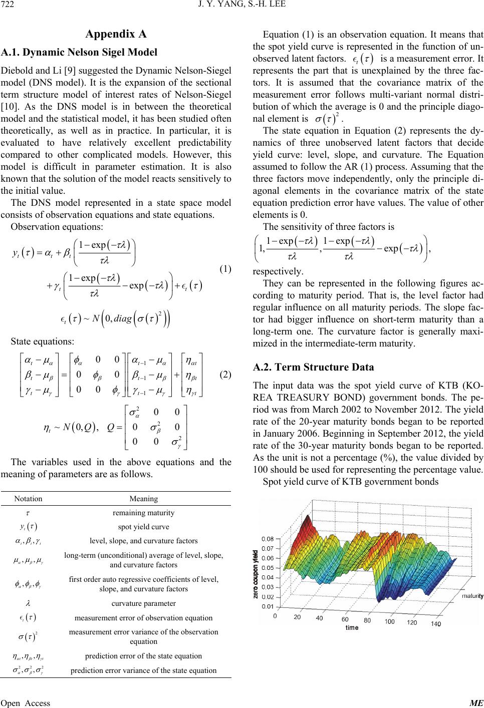

J. Y. YANG, S.-H. LEE 722
Appendix A
A.1. Dynamic Nelson Sigel Model
Diebold and Li [9] suggested the Dynamic Nelson-Siegel
model (DNS model). It is the expansion of the sectional
term structure model of interest rates of Nelson-Siegel
[10]. As the DNS model is in between the theoretical
model and the statistical model, it has been studied often
theoretically, as well as in practice. In particular, it is
evaluated to have relatively excellent predictability
compared to other complicated models. However, this
model is difficult in parameter estimation. It is also
known that the solution of the model reacts sensitively to
the initial value.
The DNS model represented in a state space model
consists of observation equations and state equations.
Observation equations:
 
  
1exp
1exp
exp
ttt
t
y

 


t

 

 


 









t
t
t


(1)
 


2
~0,
tNdiag
 
State equations:
1
1
1
00
00
00
tt
tt
tt
 
 


 







 

 
 
 
 

 







(2)

2
2
2
00
~0,, 00
00
tNQQ

















The variables used in the above equations and the
meaning of parameters are as follows.
Notation Meaning

remaining maturity


t
y

spot yield curve
,,
ttt

 level, slope, and curvature factors
,,



 long-term (unconditional) average of level, slope,
and curvature factors
,,




first order auto regressive coefficients of level,
slope, and curvature factors

curvature parameter


t

 measurement error of observation equation

2

 measurement error variance of the observation
equation
,,
ttt



 prediction error of the state equation
222
,,




prediction error variance of the state equation
Equation (1) is an observation equation. It means that
the spot yield curve is represented in the function of un-
observed latent factors.


t

 is a measurement error. It
represents the part that is unexplained by the three fac-
tors. It is assumed that the covariance matrix of the
measurement error follows multi-variant normal distri-
bution of which the average is 0 and the principle diago-
nal element is

2


.
The state equation in Equation (2) represents the dy-
namics of three unobserved latent factors that decide
yield curve: level, slope, and curvature. The Equation
assumed to follow the AR (1) process. Assuming that the
three factors move independently, only the principle di-
agonal elements in the covariance matrix of the state
equation prediction error have values. The value of other
elements is 0.
The sensitivity of three factors is




1exp 1exp
1,,exp ,
 
 
 



respectively.
They can be represented in the following figures ac-
cording to maturity period. That is, the level factor had
regular influence on all maturity periods. The slope fac-
tor had bigger influence on short-term maturity than a
long-term one. The curvature factor is generally maxi-
mized in the intermediate-term maturity.
A.2. Term Structure Data
The input data was the spot yield curve of KTB (KO-
REA TREASURY BOND) government bonds. The pe-
riod was from March 2002 to November 2012. The yield
rate of the 20-year maturity bonds began to be reported
in January 2006. Beginning in September 2012, the yield
rate of the 30-year maturity bonds began to be reported.
As the unit is not a percentage (%), the value divided by
100 should be used for representing the percentage value.
Spot yield curve of KTB government bonds
Open Access ME
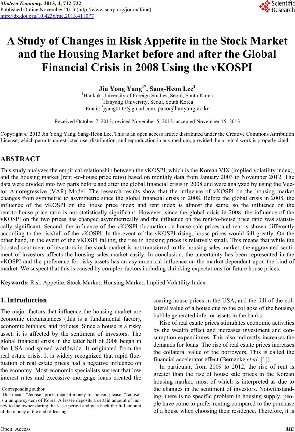