Modern Economy, 2011, 2, 1-8
doi:10.4236/me.2011.21001 Published Online February 2011 (http://www.SciRP.org/journal/me)
The Relationship between Stock Returns and Volatility in
the Seventeen Largest International Stock Markets:
A Semi-Parametric Approach
Dimitrios Dimitriou, Theodore Simos
Department of Economics, University of Ioannina, Ioannina, Greece
Received November 4, 2010; revised December 5, 2010; accepted January 1, 2011
Abstract
We empirically investigate the relationship between expected stock returns and volatility in the twelve EMU
countries as well as five major out of EMU international stock markets. The sample period starts from De-
cember 1992 until December 2007 i.e. up to the recent financial crisis. Empirical results in the literature are
mixed with regard to the sign and significance of the mean – variance tradeoff. Based on parametric GARCH
in mean models we find a weak relationship between expected returns and volatility for most of the markets.
However, using a flexible semi-parametric specification for the conditional variance, we unravel significant
evidence of a negative relationship in almost all markets. Furthermore, we investigate a related issue, the
asymmetric reaction of volatility to positive and negative shocks in stock returns confirming a negative
asymmetry in almost all markets.
Keywords: Risk-Return Tradeoff, International Stock Markets, Semi-Parametric Specification of Conditional
Variance
1. Introduction
An important topic in asset valuation research is the
tradeoff between volatility and return (typically log price
changes). The theoretical asset pricing models [1-5] link
returns of an asset to its own variance or to the covari-
ance between the returns of stock and market portfolio.
However, whether such a relationship is positive or
negative has been controversial. As summarized in [6],
most asset-pricing models [1-4] suggest a positive trade-
off for expected returns and volatility. On the other hand,
there are many empirical studies that confirm a negative
relationship between returns and volatility: [7-10]. Ref-
erence [11] indicates that there is a strong positive rela-
tionship between risk and excess return while [12,13] as
well as [9] found negative relationship in a variety of
USA market indices. Reference by [14] using data from
the S&P index, find a negative relationship between un-
expected volatility and excess returns. Similar are the
findings of [15] which use a two regime model. Accord-
ing to [14] argue that the observed negative relationship
provides indirect evidence of a positive relationship be-
tween expected risk premium and exante volatility. In
other words, if expected risk premiums are positively
related to predictable volatility, then a positive unex-
pected change in volatility increases future expected risk
premiums and lowers current stock prices. [16] also
points to a positive relationship between risk and return
for USA monthly and daily returns over the period
1926-1988. [17,18] in various assets of USA market find
a negative relationship before 1990. [19] reports no sig-
nificant relationship in USA stock market at the same
period. Also, [20] suggests that the relationship between
risk and return may be time varying. These conflicting
empirical results in the literature warrant further exami-
nation using different and probably more appropriate
econometric techniques.
In this work we utilize a flexible functional form to
model conditional variance. We favour this approach,
given that estimation via a parametric GARCH-M model
is prone to model misspecifications. Consistent estima-
tion of a GARCH-M model requires that the full model
is correctly specified [21]. Indeed, the problem that in-
ferences drawn on the basis of GARCH-M models may
be susceptible to model misspecification is well known
to applied researchers. [18] argues that parameter restric-

D. DIMITRIOS ET AL.
2
tions imposed by GARCH models may unduly restrict
the dynamics of the conditional variance process. In con-
trast, a semi-parametric specification of the conditional
variance allows flexible functional forms, and therefore
can lead potentially to more reliable estimation and in-
ference. In this paper, we propose three parametric
GARCH-M models and a semi-parametric model for
testing the null hypothesis of zero GARCH in mean ef-
fect. We then apply the above models to daily empirical
data of seventeen largest international stock markets and
two world indices. We show some evidence that a sig-
nificant negative relationship between stock market re-
turns and market volatility prevails in most major stock
markets.
Moreover the paper investigates the asymmetric im-
pact of positive and negative shocks on volatility using
two parametric models: EGARCH-M and AGARCH-M.
[21-23] provide thorough surveys in this area.
The rest of this paper is organized as follows. Section
two discusses the parametric and semi-parametric mod-
els used in the present empirical analysis, section three
presents the data, in section four we test the forecasting
power of each model, in section five we interpret the
empirical results and in section six we conclude the pa-
per.
2. The Parametric GARCH-M Model with t
Distributed Innovations
The model is specified as follows:
2
1
k
tststt
s
y
by u 


 
 (1)
ttt
u

  (2)

1..0, , , tt t
td v 

 (3)
22
11
11
.
qp
titit
ii
a







 

(4)
The dependent variable t
y denotes the stock market
returns, 2
t

their conditional variance and t u the dis-
turbance term. We assume that the random term t

is
distributed as the student’s t with ν degrees of freedom.
Equation (1) represents dynamic changes in the mean
returns, while Equation (4) describes time variation in
the conditional variance. The information available at
period t-1 is denoted by 1t
. The conditional variance
2
t

in (4), is modelled according to ARCH – GARCH
(q, p) specification of [24]. Among all the parameters to
be estimated, the most relevant for this study is the pa-
rameter δ. The sign and significance of the parameter
defines the relationship between stock market returns and
conditional variance. Setting 1
ii
a

 implies a
highly persistent conditional variance. This model is
known as the integrated GARCH or ΙGARCH which is
more likely for daily data series.
2.1. Parametric ΕGARCH-M Model
In this case the model is specified as follows:
2
1
k
tststt
s
y
by u 




 (5)
,
ttt
u



(6)


1..0,1, tt nd


 (7)
 
2
012
1
2
1
log
log.
p
ti titit
i
p
iti
i
aa E







 



(8)
The EGARCH specification allows the conditional
variance process to respond asymmetrically to positive
and negative shocks. This is reflected in the value of the
parameter product 1i

 . When


10 0 i
 , the
variance tends to rise (fall) when the shock is negative
(positive).
2.2. The Asymmetric GARCH-M (GJR) Model
In order to capture the asymmetric impact of new infor-
mation on volatility [25] suggested the GJR-GARCH (q,
p) model. It is specified by the following equations:
2
1
k
tststt
s
y
by u 




 (9)
,
ttt
u



(10)


1..0, , , tt t
td v 

 (11)
222
1211 1
11
.
qp
titttit
ii
aD

 

 

 

(12)
The conditional variance equation (12) includes an ex-
tra term: the dummy variable 1t
D, it is equal to one
when 1t


is negative (good news), and equal to zero
when 1t


is positive (bad news). A statistically sig-
nificant parameter 2

indicates volatility clustering. In
case 20

 there are leverage effects while when
20


the news impact curve is symmetric, i.e. past
positive shocks have the same impact as past negative
shocks on today’s volatility.
2.3. A Semi-Parametric GARCH-M
Specification
We consider the following semi-parametric GARCH-M

D. DIMITRIOS ET AL.
3
model
2
011 , tttttt
y
aayuxau 

  (13)
where t y is the stock market returns,

2
1
1, ,
ttt
xy


,

01
,, 'aaa

 is a vector of parameters to be estimated,

2
1
var
ttt
y 

 is the conditional on 1t  variance
of t y, 1t  is the information set available up to time
t – 1. The error term is a martingale difference process,
i.e.,

10 tt
Eu  . We are interested in testing the null
hypothesis of 0:0H

 versus 1:0H

. The null
hypothesis implies that the conditional variance 2
t

does not affect the returns t y. We first examine a simple
semi-parametric GARCH model of the form

22
11
,
ttt
mu 

 (14)
where the functional form of

m is not necessary
specified parametrically. In case

2
11tt
mua u 


the model is reduced to the standard GARCH(1,1) speci-
fication. Under the null 0:0H

 using (13), we ob-
tain 11012tt t
uyaay
 
 . Then, we can generalize (14)
as follows


22
1121
var, ,
tttt tt
yIgy y 

 (15)
where
 
1210121
,
tttt t
gyymyaay mu
 

Expression (15) allows the conditional variance to de-
pend on lagged values of t
y. Denoting


112
,
ttt
zyy


and substituting (15) recursively yields
 

22
12 3
1
tt tt
d
td
g
zgzgz
gz





 
 
(16)
Given that 0 < γ < 1, we may approximate (16) by a
finite lag model of length d:
 

22
12 3
1
tt tt
d
td
g
zgzgz
gz





 

(17)
Equation (17) is a restricted additive model with the
restriction that the different additive functions


g

are
proportional to each other. The model allows lagged
ts
y being included at the right-hand side of (17). [26],
in a similar framework, suggests a kernel-based method
to estimate the model. Although Equation (17) is only a
two-dimensional non-parametric model, it can be diffi-
cult to estimate by the popular kernel method, especially
when d is large. Moreover, when d is large, the kernel
method can give quite unreliable estimates due to its
failure to impose the additive model structure. In this
work we opt to estimate (17) by the non-parametric se-
ries method. The advantage of using a series method is
that the additive proportional model structure is imposed
directly and the estimation is performed in one step. To
this end, let
 
0
ii
y 


denote a series-based func-
tion that can be used to approximate any univariate func-
tion


my. We can use a linear combination of the
product base function to approximate

12
,
tt
gy y

,
 
 
 
 
 
''1
0'0
00 001001
10 101011
001
1
..
,
qq
iiit sits
ii
tstsqts qts
tstsqtsqts
q qtsts
qqqt sqt s
iea yy
ay yay y
ayya yy
ay y
ay ys

 
 










 





1,, .d
After re-arranging terms, the approximating function
is of the form:

 

 


21
00001
1
1
00 1
1
1
1010 1
1
1
111
1
1
001
1
1
ds
ttsts
s
ds
qtsqts
s
ds
ts ts
s
ds
qtsqts
s
ds
qqtsts
s
s
qqqt sqt s
ayy
ayy
ayy
ayy
ayy
ayy

 
 
 
 
 

































1
1
.
d
s

(18)
There are

2
11q

 parameters, namely γ and


,0,,
ij
aij q. Note that the number of parameters in
model (18) does not depend on the number of lags in-
cluded in the model. For example, if q is fixed, then the
number of parameters is also fixed. Therefore, we can let
d as T (with0dT). Asymptotically, it
allows an infinite lag structure without the curse of di-
mensionality problem (since q is independent of d). The
estimation procedure is as follows: Under 0:0H


we obtain 011ttt yaay u


. Define

0tt
y
ya


11t
ay


, then



22
1ttt
Ey


 and

2,
ttt
y
v 

 (19)
where



2
10 tt
Ey 

. Using the series approximation
of 2
t

in (18) we substitute out 2
t

in (19), and re-
placing 0 a and 1 a by the least squares estimators of
0
a and 1 a, we can estimate the parameters γ and ij a’s
using nonlinear least squares methods. Alternatively, one
can estimate ij a, 0,1, ,i, j =q, by least squares, re-
gressing 2
t
y
(

2
t
y) on the series approximating base
functions, and searching over the grid


0, 1   for op-
timizing values. In order to ensure that the above pro-

D. DIMITRIOS ET AL.
4
cedure leads to a consistent estimate of the


g

func-
tion, we need to let q and 0qT as T.
The condition q ensures that the asymptotic bias
goes to zero. For example, if one uses power series as the
base function, then it is well known that the approxima-
tion error of using a q-th order polynomial goes to zero
as q. The condition 0qT ensures that the
estimation variance goes to zero as sample increases. See
[27,28] for more details on the rate of convergence of
series estimation.
Let

2
t

denote the resulting nonparametric series es-
timator of 2
t

. Replacing 2
t

by

2
t

in Equation
(13), we get

2
011 ,
tttt
yaay



  (20)
where


2
2t
tt t
u

  . We then estimate the pa-
rameters vector

01
,, 'aaa

 by least squares. Equa-
tion (20) contains a non-parametrically generated re-
gressor

2
t

. Let


01
ˆ
,, 'aaa

 denote the resulting
estimator. If one estimate the conditional variance ignor-
ing the additive structure of 2
t

, then can use the results
of [30] and obtain the asymptotic distribution of

a
from:



0,na aN (21)
where  is the asymptotic covariance matrix. Based on
the least squares estimation of (18), the non-parametric
estimator

2
t

, is consistent under the null hypothesis
of 0:0H

.
Next, we discuss the selection of the number of lags d
and the order of series approximation q, in finite sample
applications. For a fixed value of q, the number of pa-
rameters to be estimated is fixed and does not depend on
d. In particular, choosing a large value of d does not lead
to over fitting because the number of parameters that
need to be estimated does not vary as d increases.
Therefore, it makes sense to select the value of q that
minimizes the AKAIKE information criteria.
3. Description of the Data
To estimate the models we use daily US-dollar denomi-
nated returns1 on stock indices of seventeen countries:
the twelve stock markets of the European Monetary Un-
ion, Italy (ITA), Greece (GRE), Germany (GER), France
(FRA), Finland (FIN), Belgium (BEL), Austria (AUS),
Ireland (IRL), Netherlands (NETH), Luxemburg (LUX),
Spain (SPN), Portugal (POR), as well as the United
States of America (USA), the United Kingdom (UK),
Japan (JAP), Sweden (SWD) and Russia (RUS). We also
include two world stock-indices: the international index
of DataStream’s stock-exchange markets (D-W.I.) (this
includes stocks from the most developed markets world-
wide and it remains through many years one of the most
recognized indices in the world) and the M.S.C.I (Mor-
gan Stanley Capital International) world index, which is
a stock index of the international market. The last index
includes stocks from 23 developed markets. It is com-
puted since 1969 and has been a common evaluation
index of the international stock-markets.
The data set starts from 4th December of 1992 and end
up at 5th December of 2007, comprising 3.914 observa-
tions. The source is the DataStream database. Daily re-
turns of each country are calculated using the first loga-
rithmic differences of general indices that include divi-
dends.
4. Forecasting Power of the Models
In this section we empirically investigate the four models,
stated in Section 2, in terms of their forecasting ability.
The test statistic is the mean absolute error (MAE) which
is a measurement of the co-cumulative forecasting error
of the model. In our analysis the MAE is calculated from
the monthly sub-samples of observations. Therefore, we
are able to obtain a MAE figure for each month. The
results are presented on Table 1. We notice that the best
forecasting model is the semi-parametric. In almost all
markets the average MAE of the semi-parametric model
is smaller of that of the parametric models. The second
best forecasting model is EGARCH except of Japan and
Italy where the GARCH-M and AGARCH- M models
provide a smaller MAE. Moreover, the models GARCH-M
and AGARCH-M have a similar forecasting ability with
AGARCH-M being slightly ahead. Based on the results
reported in Table 1 we conclude that forecasting ability
of the semi-parametric model is broadly superior.
5. Empirical Results
Notice that the conditional variance of the returns for
each market is calculated using the stock returns instead
of the excess stock returns. The excess return of a stock
is defined as the difference between return and the
risk-free rate that is dominant in the market. [6,18,29,30]
agree that using returns is broadly equivalent with excess
returns. In the present study for the estimation of the
conditional variance we use returns computed by log
price differences. For the three models: GARCH-M,
EGARCH-M, and AGARCH-M, we decide the appro-
priate distribution and number of lags p and q based on
the AKAIKE criterion. So, for the models GARCH-M
1As suggested by [31], calculating the returns in U.S. dollars eliminates
the local inflation.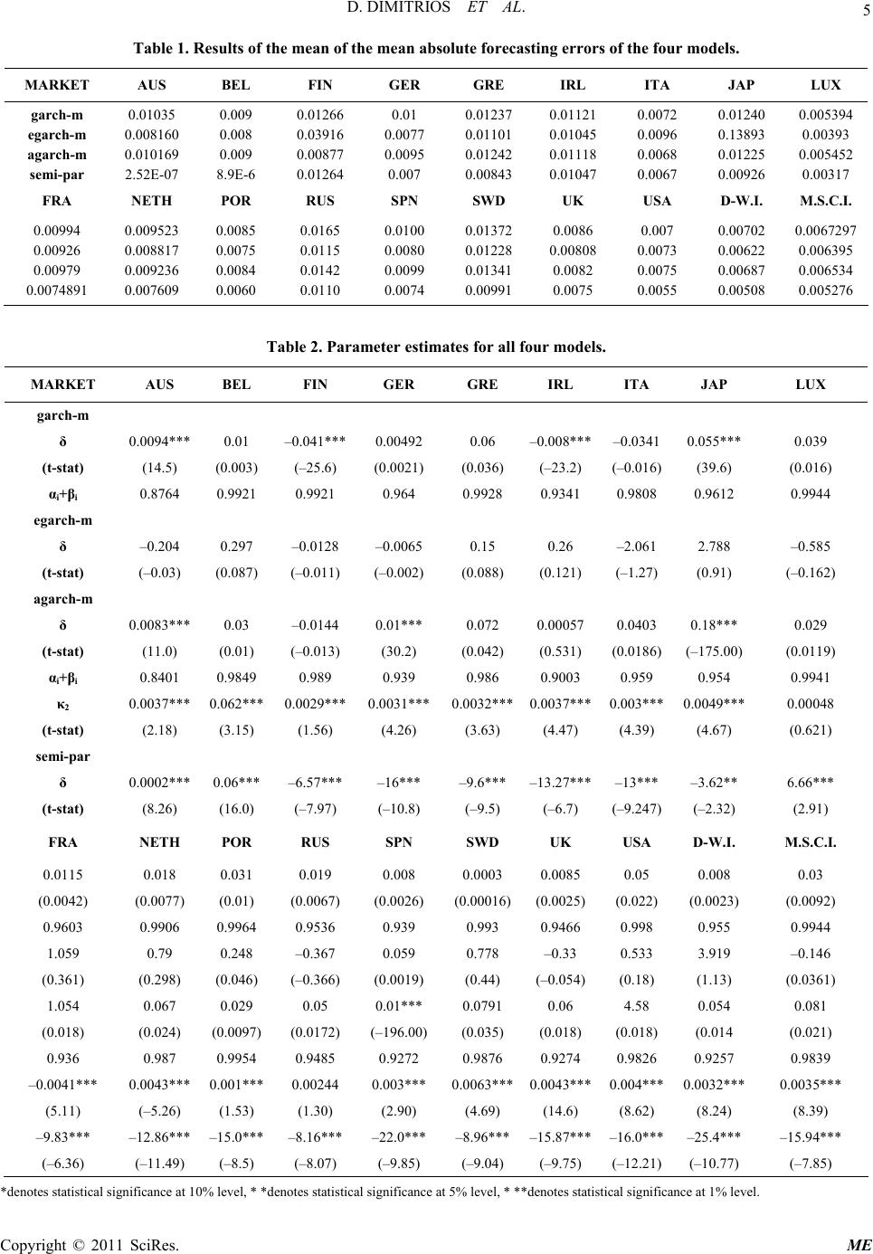

D. DIMITRIOS ET AL.
5
Table 1. Results of the mean of the mean absolute forecasting errors of the four models.
MARKET AUS BEL FIN GER GRE IRL ITA JAP LUX
garch-m
egarch-m
agarch-m
semi-par
0.01035
0.008160
0.010169
2.52E-07
0.009
0.008
0.009
8.9E-6
0.01266
0.03916
0.00877
0.01264
0.01
0.0077
0.0095
0.007
0.01237
0.01101
0.01242
0.00843
0.01121
0.01045
0.01118
0.01047
0.0072
0.0096
0.0068
0.0067
0.01240
0.13893
0.01225
0.00926
0.005394
0.00393
0.005452
0.00317
FRA NETH POR RUS SPN SWD UK USA D-W.I. M.S.C.I.
0.00994
0.00926
0.00979
0.0074891
0.009523
0.008817
0.009236
0.007609
0.0085
0.0075
0.0084
0.0060
0.0165
0.0115
0.0142
0.0110
0.0100
0.0080
0.0099
0.0074
0.01372
0.01228
0.01341
0.00991
0.0086
0.00808
0.0082
0.0075
0.007
0.0073
0.0075
0.0055
0.00702
0.00622
0.00687
0.00508
0.0067297
0.006395
0.006534
0.005276
Table 2. Parameter estimates for all four models.
MARKET AUS BEL FIN GER GRE IRL ITA JAP LUX
garch-m
δ 0.0094*** 0.01 –0.041***0.00492 0.06 –0.008***–0.0341 0.055*** 0.039
(t-stat) (14.5) (0.003) (–25.6) (0.0021) (0.036) (–23.2) (–0.016) (39.6) (0.016)
αi+βi 0.8764 0.9921 0.9921 0.964 0.9928 0.9341 0.9808 0.9612 0.9944
egarch-m
δ –0.204 0.297 –0.0128 –0.0065 0.15 0.26 –2.061 2.788 –0.585
(t-stat) (–0.03) (0.087) (–0.011) (–0.002) (0.088) (0.121) (–1.27) (0.91) (–0.162)
agarch-m
δ 0.0083*** 0.03 –0.0144 0.01*** 0.072 0.00057 0.0403 0.18*** 0.029
(t-stat) (11.0) (0.01) (–0.013) (30.2) (0.042) (0.531) (0.0186) (–175.00) (0.0119)
αi+βi 0.8401 0.9849 0.989 0.939 0.986 0.9003 0.959 0.954 0.9941
κ2 0.0037*** 0.062*** 0.0029***0.0031***0.0032***0.0037***0.003*** 0.0049*** 0.00048
(t-stat) (2.18) (3.15) (1.56) (4.26) (3.63) (4.47) (4.39) (4.67) (0.621)
semi-par
δ 0.0002*** 0.06*** –6.57***–16*** –9.6*** –13.27***–13*** –3.62** 6.66***
(t-stat) (8.26) (16.0) (–7.97) (–10.8) (–9.5) (–6.7) (–9.247) (–2.32) (2.91)
FRA NETH POR RUS SPN SWD UK USA D-W.I. M.S.C.I.
0.0115 0.018 0.031 0.019 0.008 0.0003 0.0085 0.05 0.008 0.03
(0.0042) (0.0077) (0.01) (0.0067) (0.0026) (0.00016)(0.0025)(0.022) (0.0023) (0.0092)
0.9603 0.9906 0.9964 0.9536 0.939 0.993 0.9466 0.998 0.955 0.9944
1.059 0.79 0.248 –0.367 0.059 0.778 –0.33 0.533 3.919 –0.146
(0.361) (0.298) (0.046) (–0.366) (0.0019) (0.44) (–0.054)(0.18) (1.13) (0.0361)
1.054 0.067 0.029 0.05 0.01*** 0.0791 0.06 4.58 0.054 0.081
(0.018) (0.024) (0.0097) (0.0172) (–196.00) (0.035) (0.018) (0.018) (0.014 (0.021)
0.936 0.987 0.9954 0.9485 0.9272 0.9876 0.9274 0.9826 0.9257 0.9839
–0.0041*** 0.0043*** 0.001*** 0.00244 0.003*** 0.0063***0.0043***0.004*** 0.0032*** 0.0035***
(5.11) (–5.26) (1.53) (1.30) (2.90) (4.69) (14.6) (8.62) (8.24) (8.39)
–9.83*** –12.86*** –15.0*** –8.16***–22.0*** –8.96***–15.87***–16.0*** –25.4*** –15.94***
(–6.36) (–11.49) (–8.5) (–8.07) (–9.85) (–9.04) (–9.75) (–12.21) (–10.77) (–7.85)
*denotes statistical significance at 10% level, * *denotes statistical significance at 5% level, * **denotes statistical significance at 1% level.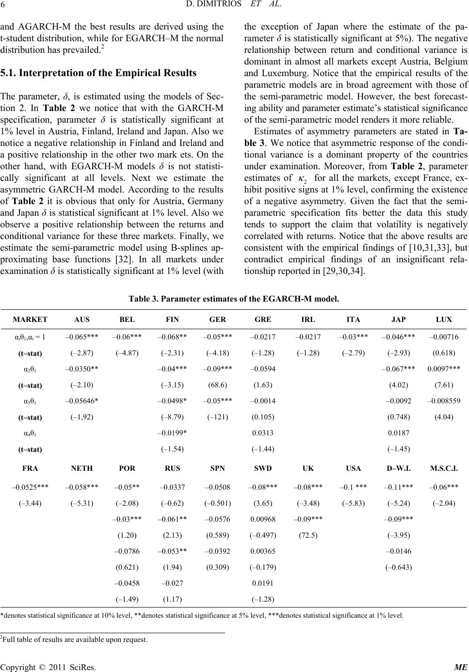

D. DIMITRIOS ET AL.
6
and AGARCH-M the best results are derived using the
t-student distribution, while for EGARCH–M the normal
distribution has prevailed.2
5.1. Interpretation of the Empirical Results
The parameter, δ, is estimated using the models of Sec-
tion 2. In Table 2 we notice that with the GARCH-M
specification, parameter δ is statistically significant at
1% level in Austria, Finland, Ireland and Japan. Also we
notice a negative relationship in Finland and Ireland and
a positive relationship in the other two mark ets. On the
other hand, with EGARCH-M models δ is not statisti-
cally significant at all levels. Next we estimate the
asymmetric GARCH-M model. According to the results
of Table 2 it is obvious that only for Austria, Germany
and Japan δ is statistical significant at 1% level. Also we
observe a positive relationship between the returns and
conditional variance for these three markets. Finally, we
estimate the semi-parametric model using B-splines ap-
proximating base functions [32]. In all markets under
examination δ is statistically significant at 1% level (with
the exception of Japan where the estimate of the pa-
rameter δ is statistically significant at 5%). The negative
relationship between return and conditional variance is
dominant in almost all markets except Austria, Belgium
and Luxemburg. Notice that the empirical results of the
parametric models are in broad agreement with those of
the semi-parametric model. However, the best forecast-
ing ability and parameter estimate’s statistical significance
of the semi-parametric model renders it more reliable.
Estimates of asymmetry parameters are stated in Ta-
ble 3. We notice that asymmetric response of the condi-
tional variance is a dominant property of the countries
under examination. Moreover, from Table 2, parameter
estimates of 2

for all the markets, except France, ex-
hibit positive signs at 1% level, confirming the existence
of a negative asymmetry. Given the fact that the semi-
parametric specification fits better the data this study
tends to support the claim that volatility is negatively
correlated with returns. Notice that the above results are
consistent with the empirical findings of [10,31,33], but
contradict empirical findings of an insignificant rela-
tionship reported in [29,30,34].
Table 3. Parameter estimates of the EGARCH-M model.
MARKET AUS BEL FIN GER GRE IRL ITA JAP LUX
αiθ1,αi = 1 –0.065*** –0.06*** –0.068** –0.05*** –0.0217 –0.0217 –0.03*** –0.046*** –0.00716
(t–stat) (–2.87) (–4.87) (–2.31) (–4.18) (–1.28) (–1.28) (–2.79) (–2.93) (0.618)
α2θ1 –0.0350** –0.04*** –0.09*** –0.0594 –0.067*** 0.0097***
(t–stat) (–2.10) (–3.15) (68.6) (1.63) (4.02) (7.61)
α3θ1 –0.05646* –0.0498* –0.05*** –0.0014 –0.0092 –0.008559
(t–stat) (–1,92) (–8.79) (–121) (0.105) (0.748) (4.04)
α4θ1 –0.0199* 0.0313 0.0187
(t–stat) (–1.54) (–1.44) (–1.45)
FRA NETH POR RUS SPN SWD UK USA D–W.I. M.S.C.I.
–0.0525*** –0.058*** –0.05** –0.0337 –0.0508 –0.08*** –0.08*** –0.1 *** –0.11*** –0.06***
(–3.44) (–5.31) (–2.08) (–0.62) (–0.501) (3.65) (–3.48) (–5.83) (–5.24) (–2.04)
–0.03*** –0.061** –0.0576 0.00968 –0.09*** –0.09***
(1.20) (2.13) (0.589) (–0.497) (72.5) (–3.95)
–0.0786 –0.053** –0.0392 0.00365 –0.0146
(0.621) (1.94) (0.309) (–0.179) (–0.643)
–0.0458 –0.027 0.0191
(–1.49) (1.17) (–1.28)
*denotes statistical significance at 10% level, **denotes statistical significance at 5% level, ***denotes statistical significance at 1% level.
2Full table of results are available upon request.

D. DIMITRIOS ET AL.
7
6. Conclusions
In this paper we empirically investigated the relationship
between expected returns and conditional variance in
twelve stock markets of the European Union as well as
five large stock markets and two world indices. Most
asset pricing models [1-4] predict a positive risk- return
tradeoff. In order to investigate this, both parametric and
semi-parametric estimation methods of the conditional
variance have been applied to daily data from the above
markets. Based on the semi-parametric specification, we
find a statistically significant negative relationship of the
risk-return tradeoff in most markets. There are only three
exceptions: Austria, Belgium and Luxemburg. Further-
more, we find significant evidence of a negative asym-
metry in almost all markets confirming the previous em-
pirical findings.
7. Acknowledgements
We wish to thank an anonymous referee of this Journal
for his/her useful comments, which improved the paper.
The usual disclaimer applies.
8. References
[1] W. F. Sharpe, “Capital Asset Prices: A Theory of Market
Equilibrium under Conditions of Market Risk,” Journal
of Finance, Vol. 19, No. 3, September 1964, pp. 425-442.
doi:10.2307/2977928
[2] J. Linter, “The Valuation of Risky Assets and the Selec-
tion of Risky Investments in Stock Portfolios and Capital
Budgets,” Review of Economics and Statistics, Vol. 47,
No. 1, February 1965, pp. 13-37.
doi:10.2307/1924119
[3] J. Mossin, “Equilibrium in a Capital Asset Market,” Eco-
nometrica, Vol. 34, No. 4, October 1966, pp. 768-783.
doi:10.2307/1910098
[4] R. C. Merton, “An Intertemporal Capital Asset Pricing
Model,” Econometrica, Vol. 41, No. 5, September 1973,
pp. 867-887. doi:10.2307/1913811
[5] R. C. Merton, “On Estimating the Expected Return on the
Market: An Exploratory Investigation,” Journal of Fi-
nancial Economics, Vol. 8, No. 4, 1980, pp. 323-361.
doi:10.1016/0304-405X(80)90007-0
[6] R. T. Baillie and R. P. DeGennaro, “Stock Returns and
Volatility,” Journa1 of Financia1 and Quantitative Ana-
1ysis, Vol. 5, No. 2, June 1990, pp. 203-214.
[7] F. B1ack, “Studies of Stock Price Volatility Changes,”
Proceedings of the 1976 Meeting of Business and Eco-
nomics Statistics Section of the American Statistical As-
sociation, Vol. 27, 1976, pp. 399-418.
[8] J. Cox and S. Ross, “The Valuation of Options for Alter-
native Stochastic Process,” Journa1 of Financia1 Eco-
nomics, Vol. 3, No.1-2, 1976, pp. 145-166.
[9] G. Bakaert and G. Wu, “Asymmetric Volatility and Risk
In Equity Markets,” Review of Financial Studies, Vol. 13,
No. 1, 2000, pp. 1-42. doi:10.1093/rfs/13.1.1
[10] R. Whitelaw, “Stock Market Risk and Return: An Em-
pirical Equilibrium Approach,” Review of Financial
Studies, Vol. 13, No. 3, 2000, pp. 521-547.
doi:10.1093/rfs/13.3.521
[11] R. Pindyck, “Risk, Inflation and the Stock Market,”
American Economic Review, Vol. 74, 1984, pp. 335-351.
[12] R.J. Shiller, “Do Prices Move too Much to be Justified by
Subsequent Changes in Dividends,” American Economic
Review, Vol. 71, No. 3, June 1981, pp. 421-436.
[13] J. Poterba and L. Summers, “The Persistence of Volatility
and Stock Market Fluctuations,” American Economic Re-
view, Vol. 76, No. 5, 1986, pp. 1142-1151.
[14] K. R. French, G. W. Schwert and R. F. Stambaugh, “Ex-
pected Stock Returns and Volatility,” Journal of Finan-
cial Economics, Vol. 19, No. 1, 1987, pp. 3-30.
doi:10.1016/0304-405X(87)90026-2
[15] H. A. Shawky and A. Marathe, “Expected Stock Returns
and Volatility in a Two Regime Market,” The Journal of
Economics and Business, Vol. 47, No. 5, December 1995,
pp. 409-422. doi:10.1016/0148-6195(95)00035-6
[16] J. Y. Campbell and L. Hentschel, “No News is Good
News: An Asymmetric Model of Changing Volatility in
Stock Returns,” Journal of Financial Economics, Vol. 31,
No. 3, 1992, pp. 281-318.
doi:10.1016/0304-405X(92)90037-X
[17] E. F. Fama and W. G. Schwert, “Asset Returns and Infla-
tion,” Journal of Financial Economics, Vol. 5, No. 2, 19-
77, pp. 115-146.
[18] D. Nelson, “Conditional Heteroscedasticity in Asset Re-
turns: A New Approach,” Econometrica, Vol. 59, No. 2,
March 1991, pp. 347-370. doi:10.2307/2938260
[19] K. C. Chan, A. Karolyi and R. Stulz, “Global Financial
Markets and the Risk Premium on US Equity,” Journal of
Financial Economics, Vol. 32, No. 2, 1992, pp. 137-167.
doi:10.1016/0304-405X(92)90016-Q
[20] C. R. Harvey, “Time-Varying Conditional Covariances in
Tests of Asset Pricing Models,” Journal of Financial
Economics, Vol. 24, No. 2, 1989, pp. 289-317.
doi:10.1016/0304-405X(89)90049-4
[21] Τ. Bollers1ev, R. Y. Chou and K. F. Kroner, “ARCH
Modeling in Finance: A Review of the Theory and Em-
pirical Evidence,” Journal of Econometrics, Vol. 52, No.
1-2, 1992, pp. 5-59.
[22] T. Bollerslev, R. F. Engle and D. B. Nelson, “ARCH
Models,” In: R. F. Engle and D. McFadden, Eds., Hand-
book of Econometrics, North-Holland, Vol. 4, 1994, pp.
2959-3038.
[23] H. Ludger, “All in the Family Nesting Symmetric and
Asymmetric GARCH Models,” Journal of Financial
Economics, Vol. 39, No. 1, September 1995, pp. 71-104.
doi:10.1016/0304-405X(94)00821-H
[24] Τ. Bollerslev, “Generalized Autoregressive Conditional
Heteroscedasticity,” Journa1 of Econometrics, Vol. 31,

D. DIMITRIOS ET AL.
8
No. 3, 1986, pp. 307-327.
[25] R. F. Eng1e and V. K. Ng, “Measuring and Testing the
Impact of News on Volatility,” Journa1 of Finance, Vol.
48, No. 5, 1993, pp. 1749-1778.
[26] L. Yang, “Direct Estimation in an Additive Model When
the Components are Proportional,” Statistica Sinica, Vol.
12, No. 3, 2002, pp. 801 -821.
[27] W. Newey, “Convergence Rates and Asymptotic Nor-
mality for Series Estimators,” Journal of Econometrics,
Vol. 79, No. 1, July 1997, pp. 147-168.
doi:10.1016/S0304-4076(97)00011-0
[28] R. De Jong, “Convergence Rates and Asymptotic Nor-
ma1ity for Series Estimators: Uniform Convergence
Rates,” Jouma1 of Econometrics, Vol. 111, No 1, 2002,
pp. 1-9.
[29] Τ. Choudhry, “Stock Market Volatility and the Crash of
1987: Evidence from Six Emerging Markets,” Journa1 of
Intemationa1 Money and Finance, Vol. 15, No. 6, 1996,
pp. 969-981.
[30] C. F. Lee, G. Chen and O. Rui, “Stock Returns and Vola-
tility on China’s Stock Markets,” Journal of Financial
Research, Vol. 24, No. 4, 2001, pp. 523-543.
[31] L. R. Glosten, R. Jagannathan and D. E. Runkle, “On the
Relation between the Expected Value and Volatility of
Nominal Excess Return on Stocks,” Journal of Finance,
Vol. 48, No. 5, 1993, pp. 1629-1658.
doi:10.2307/2329067
[32] L. L. Schumaker, “Spline Functions: Basic Theory,” Wil-
ey, New York, 1981.
[33] Q. Li, J. Yang, C. Hsiao and Y. –J. Chang, “The Rela-
tionship between Stock Returns and Volatility in Interna-
tional Stock Markets,” Journal of Empirical Finance, Vol.
12, No. 5, December 2005, pp. 650-665.
doi:10.1016/j.jempfin.2005.03.001
[34] P. Theodossiou and D. Lee, “Relationship between Vola-
tility and Expected Returns Across International Stock
Markets,” Journal of Business Finance and Accounting,
Vol. 22, No. 2, March 1995, pp. 289-300.
doi:10.1111/j.1468-5957.1995.tb00685.x