Engineering, 2013, 5, 321-325
http://dx.doi.org/10.4236/eng.2013.510B065 Published Online Octob er 2013 (http://www.scirp.org/journal/eng)
Design of a No ninvasive Bladder Urinary Volume
Monitoring System Based on Bio-Impedance
Rihui Li, Jinwu Gao, Hongbin Wang, Qing Jiang*
School of Engineering, Sun Yat-sen University, Guangzhou, China
Received July 2013
ABSTRACT
For the needs of bladder urinary volume noninvasive monitoring in clinical, we present a noninvasive bladder urinary
volume monitoring system based on bio-impedance. The system uses a four-electr ode structure, which is composed of a
pair of excitation electrodes and a pair of mea surement ele ctro des. The Direct Digital Frequency Synthesis (DDS) is
applied to generate a 50 kHz sine current excitation source. The impedance informatio n extracted from phase sensibili ty
demodulation technology is transferred to a computer through Zigbee wireless technology for real-time monitoring.
Two experiments are taken to verify the accuracy and feasib ility of the system. The experiments results show that the
system can accurately measure the corresponding electrical impedance change of the bladder. The system provides a
new way to continuously and noninvasively monito r the bladder urinary volume of patients with bladder dysfunction.
Keywords: Bio-Impedance; Bladder Urinary Volume; DDS; Zigbe e
1. Introduction
It is normal that bladder fullnes s ca uses an urge to void.
However, for some handicapped with spinal cord injury
or some p atie n ts with urological disease , this sense will
disappear, causing urinary tract infectio ns and urinary
refl ux even ultimatel y lead to renal failu re. As a result,
more and more patient s are requiring for pr ofessional
nursing, leading to the increase of the intensity of the
work staff and the p a tient’s medical costs. It is necessary
to find a way to auto matically monitor patients’ bladder
urinary volume and help them to void.
In clinic, draining urine out by a catheter inserted in
the bladder is the tra d itional method to solve this prob-
lem [1]. But this method is invasive and may cause uri-
nary tract infection. Another way to deal with this prob-
lem is to measure bladder urinary volume by using ul-
trasound. Afte r Holmes firstly measured the bladder uri-
nary volume by ultrasound in 1967, some ultrasound
instruments such as B-mode ultrasound measurement and
real time 3D ultrasound measurement were applied to
bladder volume measurement [2-4] in an imagin g way .
But the structure of ultrasound is relativel y complex and
expensive. Al though some s p ecial handheld ultrasound
bladder urinary volume measurement devices have been
developed in these years [5], all these devices are expen-
sive and unable to measure the bladder urinary volume
continuously.
Bioelectrical impedance technique is also called med-
ical electrical impedance. It extracts biomedical informa-
tion related to human’s physiological and pathological
conditions based on the electrical characteristics and va-
riation of biolo gica l tissues a nd organs. It usually applies
a small AC current or voltage to the detection object by
using an electrode system and detected the corresponding
electrical impedance changes, from wh ich we can access
to the re levant physiological and pathological informa-
tion. Long time non-invasive monitoring, high dete ction
sensitivity, rich information of function, lo w cost and
easy to use, are always the main advantages of bio-im-
pedance technology [6].
The conductivity of the bladder urine is changing dur-
ing natural bladder filling. Talibi et al. [7,8] have proved
that bladder urinary volume and electrical impedance are
closely related. The study of Liao et al. [9] has proved
that bladder urinary volume can be measured by detect-
ing the corresponding electrical impedance changes of
bladder.
In this paper, a noninvasive bladder urinary volume
monitoring system based on bio-impedance has been im-
plemented. This system, uses a four-electrode structure
and a 50 kHz sine current excitation source, measures th e
impedance information of bladder real-time with simple
operation. We have tested the accuracy of the system and
the ability to measure the bladder urinary volume to
make sure t hat the circuit structure and measurement
met hod is feasib le .
*
Corresponding author.

R. H. LI ET AL.
322
2. Syste m Design
2.1. The Measu ring Principle
Usually, the impedance characteristics of biolo gical tis-
sue can be represented by the three components equiva-
lent model [10], shown in Figure 1. Ri, Re, Cm represent
the equivalent bio lo gical tissue inner and outer resistance
and membrane capacitance.
Biological tissue shows different impedance characte-
ristics in different frequency, which can be represented
by the Cole-Cole circle diagram [11], shown in Figure 2.
Zi and Zr respectively represents the real and imaginary
part of impedance, while Z and θ respectively represent
the modulus and phase angle of impedance. Rigaud et al
[12] has proved that the imp edance characteristics of
biological tiss ue are r ich in the range of 10 kHz to 300
kHz. Therefore, the system uses a 50 kHz sine signal as
the excita tio n source.
In this paper, the system uses a four-electrode structure
whi ch is composed of a pair of excitation electrodes and
a pair of measurement electrodes. A 50 kHz sine voltage
signal is generated by a Direct Digital Frequency Syn-
thesis chip (DDS, AD9833, Analog Device Instrument).
The 50 kHz voltage signal is converted to a 50 kHz cur-
rent signal through a circuit called voltage controlle d cur-
rent source (VC CS ). The 1mA amplitude and 50 kHz
sine wave current signal is fed into the bladder through
the excitation electrodes. The instrumentation amplifier
(AD620, Analog Device Instrument) is selected to con-
stitute the front stage amplifier for extracting the small
differential voltage signal that detected by the measure-
ment electrodes. Then the amp litude of impedance ex-
tracted by a phase sensibility demodulation chip (AD8302,
Analog Device Instrument) is transferred to a computer
through Zigbee wireless technology for real-time moni-
toring.
Cm Ri
Re
Figure 1. The thr ee comp one nt s equivalent model.
Zi
Zr
Z
θ
Figure 2. Bio-impeda nc e r e spo ns e of t he ti ssue in different
frequency.
2.2. System Hardware and Software
The system is co mposed of two p a rts, including the data
acquisition module and the human-computer interaction
module. The data ac q uisition module is responsible for
measuring and transmit tin g the impedance of the bladder
while the h uma n-computer interaction module realizes
the real-time display and monitoring of Bladder imped-
ance informatio n as well as data storage function. These
two module s are communicatin g through the Zi gbee
wireless network technology. The whole system block
diagram is shown in Figure 3.
The data acquisition module is mainly composed of
three par t s.
a) The MCU (CC2530, Texas Instrument)
CC2530 is the core of the data acquisition module with
an integrate d RF wireless transceiver and a 14-bit high
accuracy A/D converter, whic h can effectively meet the
need of hardware design and simplify the circuit.
b) The excitation channel
DDS, VCCS and some peripheral components form
the excitation channel. Firstly, the DDS chip AD9833,
whi ch could dir e ctly produce sine wave current with
constant amplitude (600 mVp-p) and ad justable frequency
(0 - 12.5 MHz), is pr ogramme d to generate a 50 kHz sine
voltage signal. Eq uatio n (1) shows how to control the
frequency we want.
^
M * ( /228-1 )
out MCLK
ff=
(1)
where fMCLK is the digital clock input of AD9833 with a
25 MHz input from a crystal oscillator, M is frequency
control word, wh ich we can set it to the range of [0,
^
2 28-1
] to generate an output frequency from 0 to
12.5MHz. Then the sine wave voltage signal with 50 kHz
frequency is fed into a filtered by a high-pass filter (HP F)
who s e cut-off frequency is 2 Hz to filter the compo nents
of DC and low-frequency. Finally, the circuit called vol-
tage contro lled current source (V CCS ) converts the sine
wave voltage signal to a 1 mA amplitude and 50 kHz
sine wave current signal. The circuit of VCCS is de-
signed with two general o perational amplifiers (AD620
MCU
DDS
VCCS
R x
R ef
Gain
Detec tor
ADC
Zigbee
PC
Amp
Amp
Figure 3. Block diagram of the system. Rx represents the
impedance of bladde r , while Ref is a reference resistor.

R. H. LI ET AL.
323
and AD817, Anal og Device Instrument), which have low
noise, low drift and high p r e cisio n characteristics, to
achieve much stable sine wave current. Then the sine
wave current signal is fed into the bladder (Rx) and a
reference resistor (Ref) through a pair of excitation elec-
trodes.
c) The measurement channel
It mainly consists of differential amplifier circuits,
phase sensitive demodulation circuit and a 14-bit high
accuracy A/D conversion circuit. Firstly, two sets of tin y
voltage sig nals, one is picked up fr om the bladder and
another is picked up fro m the reference resist or, ar e re-
spectively sent to the Pin1 and Pin2 of the AD8302 after
the fro nt stage differential amplifier (AD620) amplifica-
tion process. The function of AD8302 is calculating the
differenc e of amplitude b et ween the two sets of voltage
signals. In the frequency less than 1MHz, the difference
can be calculated by Equation (2).
12
log( /)
MAGF SLPCP
VRLV VV= +
(2)
where V1 and V2 are respectively the input voltage of the
Pin1 and Pin2, VMAG is t he output corresponding to the
magnitude of the signal level differenc e, RFLSLP is 600
mV/decade or 30 mV/dB with a center-point of 900 mV
(VCP) for 0 dB gain. A range of –30 dB to +30 dB covers
the full-scale swing from 0 V to 1.8 V.
VMAG is fed into the MCU (CC2530) for A/D conver-
sion with a 14-bit high accurac y, using an external 1.8 V
voltage provided by AD8302 as a reference voltage of
A/D conversion. After the A/D conversion, the i mped-
ance of bladder can be figured out by the MCU accord-
ing to VMAG and the reference resistor. Fina lly, impedance
data is transmitted to the human-computer interactio n
module through the Zigbee wireless transmission func-
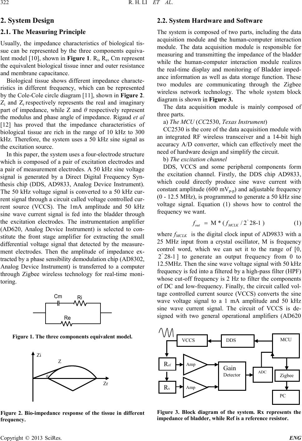
tion which is integrated into the CC2530. Figure 4
shows the prototype of the data acquisition module with
a portable design.
The human-computer interaction module consists of
two parts: the data receiving module and the monitoring
Figure 4. T he photograph of the dat a acquisition module.
sof tware. The data receiving module, which is inserted
into the computer with a USB interface, could receive the
impedance data fro m the data acquisitio n module through
the Zigbee wireless technology and tra ns mit the data to
the co mputer monitoring software. A MCU (CC2531,
Texas Instrument) is selected as the core of the data re-
ceiving module, which is integrated with Zig bee wireless
transmission function. The monitoring software is de-
veloped based on Labview. It provides the operators with
a good huma n-machine interf ace which we can observe
some impeda nce information such as how the i mpedance
changes by the increasing volume of bladder. We can
also save the measurement res ults for subsequent re-
search and analysis.
3. Experiments and Results
3.1. Accuracy of Measurem ent
As the paper mentioned above, the impedance of the
human bladder shows a downward trend as the increase
of bladder urinary volume [9]. According to previous
laboratory experiments, the impedance values of human
bladder are generally in t he range of 10 Ω - 30 Ω and the
impedance variation of the human bladder ma y be less
than 1 Ω from the beginning of accumulation of urine to
urinating. Therefore, the ability to measure a related
small amount of impedance change needs to be verified.
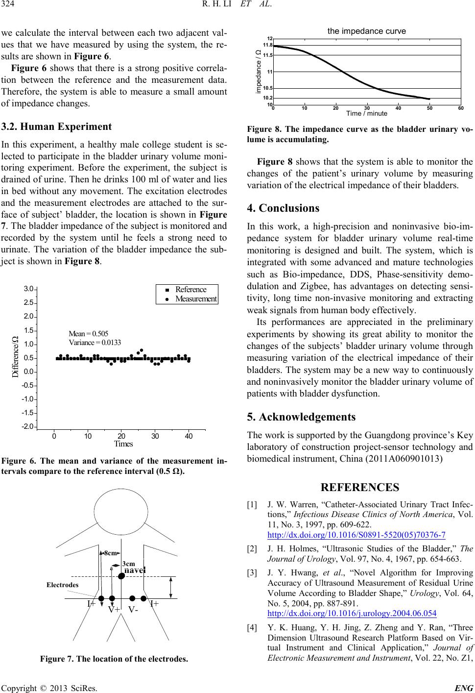
In this experiment, a varia b le resistance is selected. The
accuracy of it is 1% and the resistance value is 50 Ω. The
excitation electrodes of the system are respectively con-
nected to each end of the r esistor. The measurement
electrodes are also respectively connected to each end of
the resistor, shown in Figure 5. “A+” and “A–” represent
the excitatio n electrodes, “V+” and “V–” rep resent the
measurement electrodes.
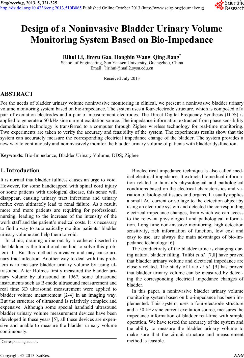
Frequency of the exciting current is 50 kHz and
peak-to-peak value is about 1 mA. From 10 Ω to 30 Ω,
we use the system to measure and record every value of
the variable resist ance with an increment of 0.5 Ω. The
Agilent E4980A Pre cisio n LCR meter with accuracy of
0.05% is use d to calibrate the variable resistance and
con fi rm that each t ime our adjustment is accurate. Then,
The
electrodes
The instrument
A+ V+V- A-
R=50Ω
Figure 5. The connection of accuracy measurement experi-
me nt .

R. H. LI ET AL.
324
we calculate the interval between each two adj acent val-
ues that we have measured by using the system, the re-
sults are shown in Figure 6.
Figure 6 shows that there is a strong po sitive cor rela-
tion between the reference and the measurement data.
Therefore, the system is ab le to measure a small amount
of impedance c hanges.
3.2. Human Experiment
In this experiment, a healthy male college student is se-
lected to particip a te in the bladder urinary volume moni-
toring experiment. Be fore the experiment, the s ubject is
drained of urine. Then he drin ks 100 ml of water and lies
in bed without any movement . The excitation electrodes
and the measurement electrodes are attached to the sur-
face of subject’ bladder, the location is shown in Figure
7. The bladder impedance of the subject is monitored and
recorded by the system until he feels a strong need to
urinate. The variation of the bladder impedance the sub-
ject is shown in Figure 8.
010 20 30 40
-2.0
-1.5
-1.0
-0.5
0.0
0.5
1.0
1.5
2.0
2.5
3.0
Times
Difference/Ω
Reference
Measurement
M ean = 0.505
Variance = 0.0133
Figure 6. The mean and variance of the me asur ement in-
tervals compare to the reference interval (0.5 Ω).
navel
V-V+ I+
I+
8cm
3cm
Electrodes
Figure 7. T he location of the electrodes.
Figure 8. The impedance curve as the bladde r ur inary vo-
lume is accumulating.
Figure 8 shows that the system is able to monitor the
changes of the patient’s urinary volume by measuring
variation of the electrical impedance of their bladders.
4. Conclusions
In this work , a high-precisio n and noninvasive bio-im-
pedance system for bladder urinary volume real-time
monitoring is designed and built. The system, which is
integrated with some advanced and mature technolo gie s
such as Bio-impedance, DD S, Phase-sens itiv ity demo-
dulation and Zigbee, has advantages on detectin g sensi-
tivity, long ti me non-invasive monitoring and extracting
weak signals from human body effectively.
Its performances are appreciated in the preliminar y
experiments by showing its great ability to monitor the
changes of the subj ects’ bladder urinary volume through
measuring variation of the electrical impedance of their
bladders. The system may be a new way to continuously
and noninvasively monitor the bladder urinary volume of
patients with bladder dysfunction.
5. Acknowledgements
The work is supported by the Guangdong province’s Key
laboratory of construction project-sensor technology and
biomedical instrument, China (2011A060901013)
REFERENCES
[1] J. W. Warren, “Catheter -Asso ciated Urinary Tract Infe c-
tions,” Infectious Disease Clinics of North America , Vol.
11, No. 3, 1997, pp. 609-622.
http://dx.doi.org/10.1016/S0891-5520(05)70376-7
[2] J. H. Holmes, “Ultrasonic Studies of the Bladder,” Th e
Journal of Urology, Vol. 97, No. 4, 1967, pp. 654-663.
[3] J. Y. Hwang, et al., “Novel Algorithm for Improving
Accurac y of Ultrasound Measu rement of Residual Urine
Volume According to Bladder Shape,” Uro log y, Vol. 64 ,
No. 5, 2004, pp. 887-891.
http://dx.doi.org/10.1016/j.urology.2004.06.054
[4] Y. K. Huang, Y. H. Jin g, Z. Zheng and Y. Ran, “Three
Dimension Ultrasound Research P latform Based on Vir-
tual Instrument and Clinical Application,” Journal of
Electronic Measurement and Instrument, Vol. 22, No . Z1,
010 20 30 40 50 60
10
10.2
10.5
11
11.5
11.8
12
the impedance c urve
Time / minute
impedance / Ω

R. H. LI ET AL.
325
2008, p. S2.
[5] H. J. Niu, et al., “Design of an Ultrasou nd Bladder Vo-
lume Measur ement and Alarm System,” 5th International
Conference on Bioinformatics and Biomedical Engineer-
ing, Wuhan, 10-12 May 2011, pp. 1-4.
[6] O. G. Martinsen and G. Sverre, “Bioimpedance and bio-
electrici ty basics,” Access Online via Elsevier, 2011.
[7] M. A. Talibi, et al., “A Model for Studying the Electrical
Stimulation of the Urinary Bladder of Dogs,” British
Journal of Urology, Vol. 42, No. 1, 1970, pp. 56-65.
http://dx.doi.org/10.1111/j.1464-410X.1970.tb11908.x
[8] F. M. Waltz, G. W. Timm and W. E. Bradley, “Bladder
Volume Sensing by Resistance Measurement,” IEEE
Transactions on Biomedical Engineering, Vol. 1, No. 1,
1971, pp. 42-46.
http://dx.doi.org/10.1109/TBME.1971.4502788
[9] W. C. Lia o and F. S. Jaw, “Noninvasive Electrical Im-
pedance Analysi s to Measure Human Urinar y Bladd er
Volume,” Journal of Obstetrics and Gynaecology Re-
search, Vol. 37, No. 8, 2011, pp. 1071-1075.
http://dx.doi.org/10.1111/j.1447-0756.2010.01487.x
[10] R. E. N. Chao-shi, “Electrical Bioimpedance Measure-
ment Technology,” China Medical Device Information,
Vol. 10, No. 1, 2004, pp. 21-25.
[11] K. S. Cole and R. H. Cole, “Dispersion and Absorption in
Dielectri cs I. Alternating Current Characteristics,” The
Journal of Chemical Physics, Vol. 9, No. 4, 1941, pp.
341. http://dx.doi.org/10.1063/1.1750906
[12] Rigaud, B., et al., “In vitro Tissue Characterizatio n and
Modeling Using Electr ical Impedance Measurements in
the 100 Hz-10 MHz Frequency Range,” Physiological
Measurement, Vol. 16, No. 3A, 1995, p. A15.