Paper Menu >>
Journal Menu >>
 Engineering, 2 http://dx.doi.or g Copyright © 2 0 Split t ABSTRA C In this paper, (GMMs) call e p roblems in o to increase t h densities foll o healthy infan t mature infant s sional Mel-F r method for tr a based re-esti m Keywords: A E x 1. Introdu c Gaussian Mi x form smooth ties and it h a model for bi o recognition s y GMMs are es t special case o gorithm base d finite amount that commit s N evertheless, antee that the r tion after eac h optimal para m p arameter est i of free para m some proble m example, in A tems using H T ting and EM - guarantee th a splitting alwa y re-estimation. in EM- b ased sensitivity to 013, 5, 277-28 3 g /10.4236/eng. 2 0 13 SciRes. t ing of G Perta i Departm e C T we make use e d adapted B o ther conventi o h e number of G o wed by learni n t s and those t h s . Cry- p attern r equency Cep s a ining GMMs m ation as a ref e A dapted Boost e x pected-Maxi m c tion x ture Model ( approximatio n a s proved to o metric syste m y stems and s p t imated from a o f the Expect a d on the max i of sample da t s tatistical err o this iterative a r e will be no d h iteration and m eters [3]. Pe r i mation error s m eters in the c l m s when incr e A utomatic Sp e T K with the m - based re-esti m a t the newly a y s increases t h Second, con v re-estimation initial para m 3 2 013.510B058 P G aussi a i ning t o H e nt of Electrica l E of the boostin g o osted Mixtur o nal technique s G aussian co m n g via the int r h at present a s e for each path o s tral Coefficie n has a better p e rence system e d Mixture Le a m ization Alg o ( GMM) has t h n s to arbitraril y be an effecti v m s, most not a p eaker identif i a vailable train a tion-Maximi z i mu m -likeliho o t a produce de t o rs in training a lgorithm co m d ecreasing in l therefore con v r formance de g s is a functio n l assifier [3], s e asing model c e ech Recogni t m ethod based o m ation [4]: F i a dded mixtur e h e likelihood f v ergence to th e is not guara n m eters of the P ublished Onlin e a n Mo d o Cry- B H esam Farsa i l Engineering, É E mail: hesam.fa r Rece i g method to i n e Learning ( B s for estimati n m ponents. The r oduced meth o e lected set of m o logical condi t n ts (MFCCs) erformance t h in multi- p ath o a rning; Gauss i o rith m ; Cry Si g h e capability t y shaped den s v e probabilis t a bly in speak i cation [1]. T h i ng data usin g z ation (EM) a o d (ML) [2]. t rimental effe c of the GM M m es with a gu a l ikelihood fun v erges to local g radation due t n of the numb o there are st i c omplexity. F o t ion (ASR) s y o n random spl i i rst, there is n e from rando m f unction prior t e optimum poi n n teed due to t h randomly sp l e October 2013 d els via B ased D i e Alaie, Ch a É colede Technol r saie-alaie.1@e n i ved June 2013 n troduce a ne w B ML). The m e n g the GMM p discriminativ e o d. Then, the G m edical condi t t ion is created feature vecto r h an the traditi o o logical classi f i an Mixture M g nals t o s i- t ic er h e g a a l- A c ts M s. ar - c- ly t o er i ll o r y s- it - n o m t o n t h e l it Gaussi a thod h a model s ture L e Marko v aforem techni q the dis c linear m this p u b een t r model mum M GM M p roach trainin g on-line newbo r which treatm e Regres s ceptro n Probab tion ( R such a s discri m (http://www.sc i Adapt e D iagnos t a kib Tadj ogy Supérieure , n s.etsmtl.ca w learning alg o e thod possess e arameters, du e e splitting ide a G MM classifie r t ions. Each gr o by using the a r . The test res u o nal method b a f ication task. M odel; Splittin g a ns. More re c a s been used t s [5,6]. Anoth e e arning (BML ) v Model (H M entioned prob l q ues for estim a c riminative s p m ixture densit i u rpose, the pa r ansformed i n as presented i M utual Inform a M s represent that enables o g (EM algori t classificatio n r n infants ca n are currently e nt. Recently s ion Neural N n (MLP), Ti m ilistic Neural N R BF) and hybr i s bagging an d m inating betw e rp.org/journal/ e e d BM L t ic Sys t , Montréal, Can a o rithm for Ga u e s the ability e in part to a n a is employed r was applied o up includes b a dapted BML m u lts demonstr a a sed upon ran d g of Gaussians ; c ently, the tr a t o solve som e e r new metho d ) to learn Ga u M M) is introd u l ems in other a a ting the GM M p litting idea h i es in a speec h a rameters of G n to their eq u n [8,9], and t h a tion (MMI) f r a statistical p o ptimal proce t hm) the clas n . Cry- b ased d n be valuable undetectable u several classi N etwork (GR N m e Delay Neu r N etwork (PN N i d systems un d d boosting [1 0 e en normal an d e ng) L Meth o t em a da u ssian Mixtur e to rectify the n ew mixing-up for Gaussian to distinguish b oth full-term m ethod and 1 3 a te that the in t d om splitting a ; a ditional boos t e p roblems o f d called Boos t u ssian mixtur e u ced to overc a vailable con v M parameters [ 4 h as been used h recognition t G aussian mo d u ivalents in l o h en trained in r amework. attern recogn i ssing of data sifier and pe r d iagnostic sy s in medical p u ntil it is too fiers such as N N), Multi-L a r al Network ( N ), Radial Ba s d er several ap p 0 ] were exa m d sick infan t ’s ENG o d e Models existing strategy mixture between and pre- 3 -dimen- t roduced a nd EM- t ing me- f mixture t ed Mix- e Hidden ome the v entional 4 ]. In [7] for log- t ask. For d el have o g-linear a Maxi- i tion ap- both for r forming s tem for p roblems late for General a yer Pe r - ( TDNN), s is Func- p roaches m ined for cry sig-  H. F. ALAIE, C. TADJ Copyright © 2013 SciRes. ENG 278 nals [11-17]. In our previous work [18], we made use of cry signals to distinguish between healthy and sick in- fants both full-term and premature. Most of the previous studies [11-17,19] concentrate on health status of infants via a binary classification task, but this paper focuses on identifying several different pathological conditions. In this article a method for splitting of Gaussian mixture densities is presented based on the boosting algorithm to maximize the frame-level ML objective function. The performed experiments on the diagnosis of infants’ dis- eases show that it has fairly superior performance to the conventional method based on random splitting and EM-based re-estimation. This paper is organized as follows: In Section 2 we give a brief review of GMM. Section 3 explains the dif- ferent parts of introduced learning algorithm. In Section 4, preprocessing steps and experiments are reported, and in section 5 a follow-up analysis of the results and a con- clusion are presented at the end to finalize this paper. 2. Gaussian Mixture M o d el A complete GMM for a D dimensional continuous value data vector called X can be represented by the weighted sum of M Gaussian component densities ,, kkk c 1, ,kM as follows: 11 ;, 1, MM Mkkkkk kk FXc Xc (1) where each mixture component k is a D-dimen- sional multivariate Gaussian distribution and ,, kkk c are the mixture weights, mean vector and covariance matrix respectively. Since GMMs are used usually in unsupervised learning and clustering problems with un- known number of mixtures and their parameters, the choice of model configuration is almost determined by the amount of data available for estimating the GMM parameters in a particular application. GMM, as a para- metric probability density function with the following adapted learning method could be a successful candidate for cry-based physical or psychological status identifica- tion system. 3. Adapted Boosted Mixture Model Generally, boosting method combines weak learners or base classifiers in a weighted majority voting scheme to improve the overall classification accuracy for almost any type of learning algorithm [20,21]. The main idea of boosting is that instead of always treating all data points as equal, component classifiers should specialize on cer- tain examples. Moreover, some recent work has shown that the boosting method can effectively increase the margin of all training samples, which can be explained by a theoretical view related to functional gradient tech- niques [4,22]. We should note that the boosting algo- rithm does not always improve the accuracy of a learning algorithm nor does it always increase the margin. In the presented method a new component k and its weight k wcan be trained based discriminatively based on a predefined objective function, denoted as , in an optimal way. Then, they will be added to the pre- vious mixture model k-1 F which has k − 1 mixture components to grow into a new mixture model k F . 1 1kkkkk F XcFcX (2) Objective function is defined as the log likelihood function of the mixture model k F , based on all training data 12 ,, T XX X. 1 log T kkt t F FX (3) where k w is a weight to combine the new mixture component with the current model. When a new mixture component k is added, it will increase the ML objec- tive function with respect to Funtil the criterion which will be explained later is met. 1 1k-1kk CεF+εN>CF (4) where is a small deviation constant. Thus, the new mixture component k should be estimated in order to increase the ML objective function the most. By em- ploying Teylor’s series and predefined inner product of mixture models p and Q over training samples, T tt t1 1 P,QP XQ X T (5) the optimal new component can be obtained by: k * kk1kk1 argmaxF ,F k Tkt t1 k1 t X argmax FX (6) The new mixture component is generated along the direction of functional gradient where the objective func- tion grows the most. There is no closed-form of the op- timization problem for GMMs, but it can be solved by optimizing a lower bound on the boosting learning for- mula with the EM algorithm [4]. After estimating * k , the mixture weight * k c can be obtained by using the following line search: ** 1 0,1 1 k kkkkk c cargmax cFc (7) 3.1. Process of Adding a New Component In this method, a single Gaussian model initialized by ML training is estimated to fit the data at first, and then  H. F. ALAIE, C. TADJ Copyright © 2013 SciRes. ENG 279 in each step it is split into two Gaussians followed by learning via introduced method. In the splitting or adding process the part of training vectors in which k X has a higher value than the reminder of the mixture mod- el, denoted by kk F is selected. Then this subset of data indicated by s ub X should be modeled by a small GMM consisting in two Gaussian components called * k and k1 . The initial component came from the EM-based re-estimation, and then the second component and its weight were estimated based upon adapted BML method. We considered the estimated component—the second one—as an initial component and run the algo- rithm again. This process continues repeatedly, until it reached the optimal maximum log-likelihood estimate of parameters over s ub X . This procedure for finding the best two new components 1k and * k continued for 1, ,kK . Amongst all the created K mixture models, denoted by 1K F , the one that gave the highest value of the objective function was selected and added to the mixture by adjusting its weight. This iterative density splitting process in ML frame work is repeated as long as the added component causes an increase in the prede- fined objective function. 3.2. Partial and Global Updating During previous step, instead of finding the new mixture weight from the line search, there is an alternative me- thod called partial updating in which each new compo- nent and its weight are estimated at the same time, which is preferable since it may result in more robust and relia- ble estimation. , ** 1 , ,1 kk kkkk kk c cargmaxcFc (8) The iterative re-estimation formula for model parame- ters n1 11 k Φ, nn kk at the th n1 iteration can be evaluated as follows: [4]: 11 1 n ktk n tn nn kktkk ktk X wX cX cFX 1 n nt tk Tn t t wX wX 1? 1 1T nnn kkt t ccwX T 1 1 . T n n ktkt t X 111 1 .? TTr n nnn ktktktk t XX (9) where n t wX denotes the weight assigned to sample t X at the th n iteration, similar to sample weights used in the traditional boosting algorithms and 1 , kkk . Moreover, in order to speed up con- verging process and finding the minimum number of Gaussian component in the final mixture, the current mixture model k F should be updated globally over training data samples before adding the next component. For example in the GMM with k components, denoted by k F , the th k component can be re-estimated for 1, ,kK when the reminder of the mixture mode is assumed to be fixed. It means that after obtaining a mix- ture model K F , we could update each component k and its weight over all training feature vectors by using the same updating equations. The parameters updating phase, subsequent to splitting the selected density in half, brings about an increase in the objective function through the localized training of each component separately. 3.3. Initialization of Sample Weights A problem may arise when the initial values of the weights are chosen by boosting theory as follow: 0 11 1/ tktk wXF X (10) The dynamic range of 1k F is large in a way that it could be dominated by only a few number of outliers or samples with low probabilities. We use the so-called “Weight decay” method [23] to overcompensate for the low probability by smoothing sample weights based on power scaling. 0 11 (1 0/1,)p tktk wXF Xp (11) where p is a decay parameter or an exponential scaling factor. In the second method the idea of sampling boost- ing in [24] is applied to form a subset of training feature vectors according to the mean and variance values of the decayed weights. Afterwards, vectors contained in the previously created subset are utilized with equal weights to estimate the new component parameters. Assume M and 2 denote the mean and variance of weights calcu- lated in equation (9) as defined below. 0 t meanlog wMX 20 t variancelog wX (12) Then, the aforementioned subset with large weights is selected as described below: 0 sub tt XXlogwXM (13) where is a linear scaling factor to control the size of subset s ub X . In the experiments, we set 0.05p and 0.5 to overcome over fitting and these same para- meter values which utilized for BML algorithm in [4].  H. F. ALAIE, C. TADJ Copyright © 2013 SciRes. ENG 280 3.4. Criterion for Model Selection The process of adding new mixture component to the previous mixture model is continued incrementally and recursively until the optimal number of mixtures is met. The set of Gaussian components selected should re- present the space covered by the feature vectors. For this purpose, the selected strategy to stop the adding process is a criterion-based called Bayesian Inference Criterion (BIC). It can be represented as the following [25]: log kk BIC kFMT (14) where k F is the log-likelihood function of the mix- ture model over all training data, k M is the number of parameters used in model k F , and T denotes total number of training data. Figure 1 shows a brief review of all mentioned processes to train a GMM for each available pathological condition in order. A simple pro- cedure to evaluate the presented learning method is to monitor the progress of the method during learning phase with a created training dataset, whose samples have been drawn from a known mixture of multivariate Gaussian distributions. Given training data with 600 two-dimen- sional samples, we wish to estimate the parameters of the GMM, ,, kkk c , which in some sense best matches the distribution of the training feature vectors. Figure 2 shows the final trained GMM and the whole discriminative splitting process after each substitution step. We compare the log-likelihood score between our method and the mentioned traditional method at the end of the discriminative training of this model. The negative log-likelihood score of the estimated GMM bears a close resemblance to that of the trained model with the tradi- tional method consisting of the correct number of Gaus- sian components on the same data, whose values are 3 2.7682 10 and 3 2.7684 10 respectively. 4. Experiments 4.1. Preprocessing and Features Extraction It would be worthwhile to find a clear correlation be- tween infants’ medical statuses and extracted cry charac- teristics. This concept could prove useful in the early infant diagnosis system. Several different cry characte- ristics and features were described in [19,26] and have Figure 1. Block diagram of adapted BML technique. been shown to work well in practice for distinguishing between a healthy infant’s cry and that of infants with asphyxia, brain damage, hyperbilirubinemia, Down’s syndrome, and mothers who abused drug during their pregnancies. Therefore, selecting the most informative features to distinguish between healthy baby class and pathological infant classes with different pathology con- ditions has a significant role in pathological classification tasks. Table 1 shows the list of available different pa- thological conditions and the number of samples in each class; totaling 63 cry signals for each healthy and sick infants classes including both full-term and premature per class. In a similar way to typical speech recognition systems, the pre-processing and the feature extraction phases are modeled in such a way that irrelevant information to phonetic content of the cries should be eliminated as far as possible i.e. nurses talking and environmental noises. On the other hand, the Mel-Frequency Cepstral Coeffi- cients (MFCCs) are selected to be extracted from the cries which contain the vocal tract information [27]. This type of excitation source characteristics is one of the popular schemes in speaker recognition and identifica- tion systems [27-30]. It is common practice to pre-em- phasis the signal prior to computing the speech parame- ters by applying the filter 1 10.97Pz z [31,32]. In all related practical applications, the short terms or frames should be utilized, which implies that the signal characteristics are uniform in the region. Prior to any frequency analysis, the Hamming windowing is neces- sary to reduce any discontinuities at the edges of the se- lected region. A common choice for the value of the window length is 10 - 30 ms [32-34]. A total number of 12 MFCCs ,1,,12 n Cn are computed directly from the data [31,35]. For better per- formance, the 0th cepstral coefficient 0 C is appended to the vector which is simply a version of energy (i.e., weighting with a zero-frequency cosine). Therefore, each frame is represented by a 13-dimensional MFCCs feature vector [33]. 4.2. Multi-Pathology Classification In training phase of algorithm, in order to estimate the parameters of GMMs for pathology classes, almost 63% of total cry signals were employed and the reminder for system evaluation. The GMM classifier is employed to identify infants’ pathological conditions. The Maximum Likelihood (ML) decision criterion is applied to assist in choosing between hypotheses. #argmax j j P athology ClassX (15) where j X shows the likelihood of a feature vector X given a Gaussian model i for th i pathology class. 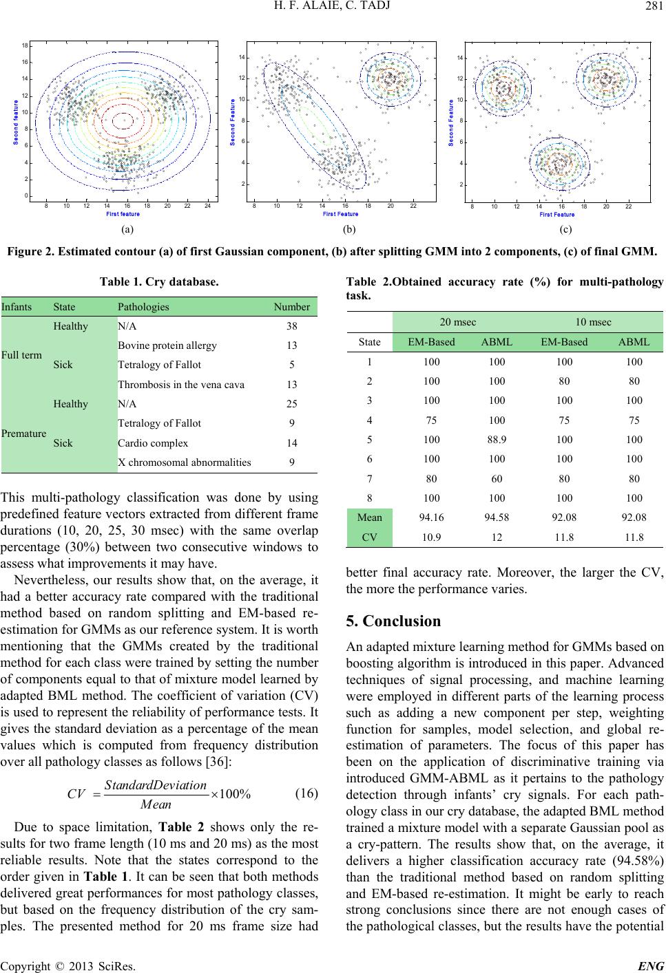 H. F. ALAIE, C. TADJ Copyright © 2013 SciRes. ENG 281 (a) (b) (c) Figure 2. Estimated contour (a) of first Gaussian component, (b) after splitting GMM into 2 components, (c) of final GMM. Table 1. Cry database. Infants State Pathologies Number Full term Healthy N /A 38 Sick Bovine protein allergy13 Tetralogy of Fallot5 Thrombosis in the vena cava13 Premature Healthy N /A 25 Sick Tetralogy of Fallot9 Cardio complex14 X chromosomal abnormalities9 This multi-pathology classification was done by using predefined feature vectors extracted from different frame durations (10, 20, 25, 30 msec) with the same overlap percentage (30%) between two consecutive windows to assess what improvements it may have. Nevertheless, our results show that, on the average, it had a better accuracy rate compared with the traditional method based on random splitting and EM-based re- estimation for GMMs as our reference system. It is worth mentioning that the GMMs created by the traditional method for each class were trained by setting the number of components equal to that of mixture model learned by adapted BML method. The coefficient of variation (CV) is used to represent the reliability of performance tests. It gives the standard deviation as a percentage of the mean values which is computed from frequency distribution over all pathology classes as follows [36]: 100% StandardDev i ation CV Mean (16) Due to space limitation, Table 2 shows only the re- sults for two frame length (10 ms and 20 ms) as the most reliable results. Note that the states correspond to the order given in Table 1. It can be seen that both methods delivered great performances for most pathology classes, but based on the frequency distribution of the cry sam- ples. The presented method for 20 ms frame size had Table 2.Obtained accuracy rate (%) for multi-pathology task. 20 msec 10 msec State EM-Based ABML EM-Based ABML 1 100 100 100 100 2 100 100 80 80 3 100 100 100 100 4 75 100 75 75 5 100 88.9 100 100 6 100 100 100 100 7 80 60 80 80 8 100 100 100 100 Mean 94.16 94.58 92.08 92.08 CV 10.9 12 11.8 11.8 better final accuracy rate. Moreover, the larger the CV, the more the performance varies. 5. Conclusion An adapted mixture learning method for GMMs based on boosting algorithm is introduced in this paper. Advanced techniques of signal processing, and machine learning were employed in different parts of the learning process such as adding a new component per step, weighting function for samples, model selection, and global re- estimation of parameters. The focus of this paper has been on the application of discriminative training via introduced GMM-ABML as it pertains to the pathology detection through infants’ cry signals. For each path- ology class in our cry database, the adapted BML method trained a mixture model with a separate Gaussian pool as a cry-pattern. The results show that, on the average, it delivers a higher classification accuracy rate (94.58%) than the traditional method based on random splitting and EM-based re-estimation. It might be early to reach strong conclusions since there are not enough cases of the pathological classes, but the results have the potential First feature Second feature 810 1214 16 18 20 2224 0 2 4 6 8 10 12 14 16 18 First Fea tu re Second Feature 810 12 1416 18 20 22 2 4 6 8 10 12 14 Fir s t Fe a tu re Second Feature 810 12 1416 18 20 22 2 4 6 8 10 12 14  H. F. ALAIE, C. TADJ Copyright © 2013 SciRes. ENG 282 to serve as a mixture learning method for further research. We are currently trying to use alternative discriminative criteria like MMI rather than ML and collecting more sample cries for further tests. 6. Acknowledgements We would like to thank Dr. Barrington and members of neonatology group of Mother and Child University Hos- pital Center in Montreal (QC) for their dedication of the collection of the Infant’s cry data base. This research work has been funded by a grant from the Bill & Melinda Gates Foundation through the Grand Challenges Explo- rations Initiative. REFERENCES [1] D. A. Reynolds and R. C. Rose, “Robust Text-Indepen- dent Speaker Identification Using Gaussian Mixture Speaker Models,” IEEE Transactions on Speech and Au- dio Processing, Vol. 3, 1995, pp. 72-83. http://dx.doi.org/10.1109/89.365379 [2] A. P. Dempster, et al., “Maximum Likelihood from In- complete Data via the EM Algorithm,” Journal of the Royal Statistical Society. Series B (Methodological), Vol. 39, 1977, pp. 1-38. [3] L. P. Heck and K. C. Chou, “Gaussian Mixture Model Classifiers for Machine Monitoring,” IEEE International Conference on Acoustics, Speech, and Signal Processing, Vol. 6, 1994, pp. VI/133-VI/136. [4] D. Jun, et al., “Boosted Mixture Learning of Gaussian Mixture Hidden Markov Models Based on Maximum Li- kelihood for Speech Recognition,” IEEE Transactions on Audio, Speech, and Language Processing, Vol. 19, 2011, pp. 2091-2100. http://dx.doi.org/10.1109/TASL.2011.2112352 [5] M. Kim and V. Pavlovic, “A Recursive Method for Dis- criminative Mixture Learning,” Proceedings of the 24th International Conference on Machine Learning, 2007, pp. 409-416. [6] V. Pavlovic, “Model-Based Motion Clustering Using Boosted Mixture Modeling,” Proceedings of the 2004 IEEE Computer Society Conferences on Computer Vision and Pattern Recognition, Vol. 1, 2004, pp. I-811-I-818. [7] W. Boyu, et al., “Gaussian Mixture Model Based on Ge- netic Algorithm for Brain-Computer Interface,” 3rd In- ternational Congress on Image and Signal Processing (CISP), 2010, pp. 4079-4083. [8] G. Heigold, et al., “Equivalence of Generative and Log- Linear Models,” IEEE Transactions on Audio, Speech, and Language Processing, Vol. 19, 2011, pp. 1138-1148. http://dx.doi.org/10.1109/TASL.2010.2082532 [9] G. Heigold, et al., “On the Equivalence of Gaussian and log-Linear HMMs,” INTERSPEECH, 2008, pp. 273-276. [10] E. Bauer and R. Kohavi, “An Empirical Comparison of Voting Classification Algorithms: Bagging, Boosting, and Variants,” Machine Learning, Vol. 36, 1999, pp. 105-139. http://dx.doi.org/10.1023/A:1007515423169 [11] M. Hariharan, et al., “Normal and Hypoacoustic Infant Cry Signal Classification Using Time-Frequency Analy- sis and General Regression Neural Network,” Computer Methods and Programs in Biomedicine, Vol. 108, 2012, pp. 559-569. http://dx.doi.org/10.1016/j.cmpb.2011.07.010 [12] M. Hariharan, et al., “Pathological Infant Cry Analysis Using Wavelet Packet Transform and Probabilistic Neural Network,” Expert Systems with Applications, Vol. 38, 2011, pp. 15377-15382. http://dx.doi.org/10.1016/j.eswa.2011.06.025 [13] E. Amaro-Camargo and C. Reyes-García, “Applying Statistical Vectors of Acoustic Characteristics for the Automatic Classification of Infant Cry,” In: D.-S. Huang, et al., Eds., Advanced Intelligent Computing Theories and Applications. With Aspects of Theoretical and Methodo- logical Issues, Vol. 4681, Springer Berlin/Heidelberg, 2007, pp. 1078-1085. [14] S. Cano, et al., “A Combined Classifier of Cry Units with New Acoustic Attributes,” In: J. Martínez-Trinidad, et al., Eds., Progress in Pattern Recognition, Image Analysis and Applications, Vol. 4225, Springer Berlin/Heidelberg, 2006, pp. 416-425. [15] O. Galaviz and C. García, “Infant Cry Classification to Identify Hypo Acoustics and Asphyxia Comparing an Evolutionary-Neural System with a Neural Network Sys- tem,” In: A. Gelbukh, et al., Eds., MICAI 2005: Advances in Artificial Intelligence, Vol. 3789, Springer, Berlin/ Heidelberg, 2005, pp. 949-958. [16] S. C. Ortiz, et al., “A Radial Basis Function Network Oriented for Infant Cry Classification,” In: A. Sanfeliu, et al., Eds., Progress in Pattern Recognition, Image Analy- sis and Applications, Vol. 3287, Springer, Berlin/Hei- delberg, 2004, pp. 15-36. [17] J. Orozco and C. A. R. Garcia, “Detecting Pathologies from Infant Cry Applying Scaled Conjugate Gradient Neural Networks,” European Symposium on Artificial Neural Networks, Bruges, 2003. [18] H. FarsaieAlaie and C. Tadj, “Cry-Based Classification of Healthy and Sick Infants Using Adapted Boosting Mix- ture Learning Method for Gaussian Mixture Models,” Modelling and Simulation in Engineering, Vol. 2012, p. 10. [19] O. Wasz-Hockert, et al., “Twenty-Five Years of Scandi- navian cry Research,” New York, 1985. [20] C. Bishop, “Pattern Recognition and Machine Learning,” Springer, Berlin, 2006. [21] R. O. Duda, et al., “Pattern Classification,” John Wiley & Sons, 2001. [22] L. Mason, et al., “Functional Gradient Techniques for Combining Hypotheses,” In: A. J. Smola, et al., Eds., Advances in Large Margin Classifiers, MIT Press, Cam- bridge, 2000, pp. 221-246. [23] S. Rosset, “Robust Boosting and Its Relation to Bagging,” Proceedings of the 11th ACM SIGKDD International Conferences on Knowledge Discovery in Data Mining, Chicago, Illinois, 2005.  H. F. ALAIE, C. TADJ Copyright © 2013 SciRes. ENG 283 [24] Y. Freund and R. E. Schapire, “A Decision-Theoretic Generalization of On-Line Learning and an Application to Boosting,” Journal of Computer and System Sciences, Vol. 55, 1997, pp. 119-139. http://dx.doi.org/10.1006/jcss.1997.1504 [25] G. Schwarz, “Estimating the Dimension of a Model,” The Annals of Statistics, Vol. 6, 1978, pp. 461-464. http://dx.doi.org/10.1214/aos/1176344136 [26] M. J. Corwin, et al., “The Infant Cry: What Can It Tell Us?” Current Problem Pediatrics, Vol. 26, 1996, pp. 325- 334. http://dx.doi.org/10.1016/S0045-9380(96)80012-0 [27] M. D. Plumpe, et al., “Modeling of the Glottal Flow De- rivative Waveform with Application to Speaker Identifi- cation,” IEEE Transactions on Speech and Audio Processing, Vol. 7, 1999, pp. 569-586. [28] W. Longbiao, et al., “Speaker Identification by Combin- ing MFCC and Phase Information in Noisy Environ- ments,” IEEE International Conference on Acoustics Speech and Signal Processing (ICASSP), 2010, pp. 4502- 4505. [29] K. S. R. Murty and B. Yegnanarayana, “Combining Evi- dence from Residual Phase and MFCC Features for Speaker Recognition,” IEEE Signal Processing Letters, Vol. 13, 2006, pp. 52-55. [30] Z. Nengheng, et al., “Integration of Complementary Acoustic Features for Speaker Recognition,” IEEE Signal Processing Letters, Vol. 14, 2007, pp. 181-184. http://dx.doi.org/10.1109/LSP.2006.884031 [31] S. Young, et al., “The HTK Book (for HTK Version 3.4),” Cambridge University Engineering Department, 2006. [32] L. R. Rabiner and R. W. Schafer, “Digital Processing of Speech Signals,” Prentice-Hall, Upper Saddle River, 1978. [33] X. Huang, et al., “Spoken Language Processing: A Guide to Theory, Algorithm, and System Development,” Pren- tice Hall, Upper Saddle River, 2001. [34] M. Benzeghiba, et al., “Automatic Speech Recognition and Speech Variability: A Review,” Speech Communica- tion, Vol. 49, 2007, pp. 763-786. http://dx.doi.org/10.1016/j.specom.2007.02.006 [35] J. John R. Deller, et al., “Discrete Time Processing of Speech Signals,” Prentice Hall, Upper Saddle River, 1993. [36] D. Zill, et al., “Advanced Engineering Mathematics,” Fourth Edition, 2011. |