Journal of Financial Risk Management
2013. Vol.2, No.4, 71-76
Published Online December 2013 in SciRes (http://www.scirp.org/journal/jfrm) http://dx.doi.org/10.4236/jfrm.2013.24012
Open Access 71
Empirical Study on Overreaction and Underreaction in Chinese
Stock Market Based on ANAR-TGARCH Model
Yong Fang1,2,3
1Post-Doctoral Scientific Research Workstation, Shanghai International Group Co., Ltd. (SIG), Shanghai, China
2Post-Doctoral Research Station for Applied Economics, Fudan University, Shanghai, China
3Department of Applied Mathematics, Shanghai Finance University, Shanghai, China
Received July 26th, 2013; August 26th, 2013; September 5th, 2013
Copyright © 2013 Yong Fang. This is an open access article distributed under the Creative Commons Attribu-
tion License, which permits unrestricted use, distribution, and reproduction in any medium, provided the original
work is properly cited.
An ANAR-TGARCH model is adopted in this paper. By using a first-order asymmetric autoregressive
mean equation, we conduct a series of robust tests on overreaction and underreaction in the Chinese stock
market by taking the abnormal value, run length, time scale, size, industry, style, and market cycle into
account. We then comprehensively compare the intensities of the first-order autocorrelation by using
Wald coefficients tests. Results could provide strong empirical support for generating stock market in-
vestment strategies.
Keywords: Overreaction; Underreaction; ANAR-TGARCH Model
Introduction
Since the mid-1980s, behavioral finance has rapidly risen
and become an entire theory system. Behavioral finance dem-
onstrates broad prospects because of its theoretical analysis of
real investment behavior, and causes significant changes in
modern financial theory structure and financial research para-
digm (Kahneman & Tversky, 1979; Thaler, 1985; De Long,
Shleifer, Summers, & Waldmann, 1990a; De Long, Shleifer,
Summers, & Waldmann, 1990b; Gervais & Odean, 2001; Bac-
chetta & Wincoop, 2008; Barberis, Huang, & Santos, 2001).
Overreaction or underreaction to information is one of the
important behavioral characteristics of investors with limited
rationale. A number of empirical studies reported that stock
returns show significant autocorrelation. Traditional financial
theory based on the rational person hypothesis cannot provide a
reasonable explanation for this phenomenon. Behavioral fi-
nance attributes the significant autocorrelation of stock returns
to the biased reaction of investors to new information, including
overreaction and underreaction. Thus, as new information ap-
pears, investors cannot revise their views according to the
Bayesian rule.
In behavioral finance theory, many classical models are used
to analyze the overreaction or underreaction of investors. Bar-
beris, Shleifer, & Vishny (1998) assumed that investors have
two kinds of mental biases when making investment decisions.
One is the representative bias, in which investors make infer-
ences and judgments according to a small sample and ignore
the population. Another is the conservative bias, in which in-
vestors are unable to update their expectations in a timely
manner according to new information. The representative bias
causes overraeaction and the conservative bias causes underre-
action to new information. Daniel, Hirshleifer, & Subrah-
manyam (1998) explained overreaction and underreaction from
another perspective. They divided all investors into informed
and uninformed investors. Uninformed investors do not have
mental biases but informed investors do. These mental biases
include overconfidence and self-attribution. Commonly over-
confident, informed investors depend excessively on private
information and underestimate the value of public information.
Such investors likewise overestimate their ability to forecast
and underestimate their forecasting error. Overconfidence can
lead to mispricing of stocks. Generally, overconfidence is usu-
ally encouraged by another mental bias, namely, self-attribution,
which is when investors attribute their success to their own
abilities and attribute failure to external noise. De Bondt &
Thaler (1985) sorted all stocks listed in the New York Stock
Exchange according to accumulated returns over the past years
and constructed two portfolios. One portfolio was called “win-
ners” and comprised 35 stocks with the best performance. The
other portfolio was called “losers” and comprised 35 stocks
with the worst performance. The accumulated returns of these
two portfolios over the next three years were then examined.
Losers were found to greatly outperform winners. Behavioral
finance can provide a feasible explanation for this phenomenon.
Investors usually overestimate the value of winners and under-
estimate the value of losers, resulting in mispricing. When mis-
pricing is corrected after a period of time, the accumulated
returns of losers would be greater than that of winners.In this
paper, an ANAR-TGARCH model is adopted to test overreac-
tion or underreaction in the Chinese stock market. A series of
robust tests were conducted on the underreaction or overreac-
tion of investors by taking run length, abnormality degree, time
scale, size, sector, style, and market cycle into account. Wald
coefficients tests are then used to compare autocorrelation in-
tensities. The empirical results in this paper could help inves-

Y. FANG
tors adopt a suitable investment strategy.
Data, Models and General Empirical Results
In this section, we use daily returns in the Shanghai Compos-
ite Index, denoted by t. The value of is calculated ac-
cording to the following formula,
rt r
1
ln ln
tt
rPP


t
, (1)
where is the daily closing price of the Shanghai Composite
Index.
t
P
The sample period is from January 2, 2001 to January 21,
2013. The sample size is 2917.
All data in this paper are derived from the Wind Financial
Terminal.
In this paper, an ANAR-TGARCH model is adopted to test
overreaction or underreaction in the Chinese stock market. The
mean equation is a first-order asymmetric autoregressive model
(ANAR), denoted by




11 11
00
ttttt
rIrr Irr
t


 
    , (2)
and the volatility equation is a TGARCH(1,1) model, denoted
by


22 2
111
0
tttt
wI 2
1t

 

 

.
(3)
Random error is assumed to follow the general error distribu-
tion (GED). Coefficient estimates are shown in Table 1, where
“*” represents the significant level of .1, “**” represents the
significant level of .05, and “***” represents the significant level
of .01 (the same below).
As shown in Table 1, both the means and volatilities of daily
returns of the Shanghai Composite Index present a significant
asymmetric pattern. Notably,

is significantly greater than 0.
Moreover,

is significantly less than 0. From the statistical
point of view, when the return at time t-1 is conditionally posi-
tive, the return at time t would present a significant positive
first-order autocorrelation. When the return at time t-1 is condi-
tionally negative, the return at time t would present a significant
negative first-order autocorrelation. From the behavioral point
of view, investors underreact to good news and overreact to bad
news.
The empirical results above can provide a significance refer-
ence with regard to which type of investment strategy to adopt.
When the previous period return is conditionally positive, one
could adopt a tendency strategy. When the previous period
return is conditionally negative, one could adopt a contrarian
strategy.
Table 1.
Coefficient estimates of the ANAR-TGARCH model for daily returns
of Shanghai Composite Index.
Coefficient Estimate P value of z-test

.071478 .0027***

−.069902 .0048***
w .000004 .0007***

.046011 .0001***

.037920 .0059***

.920696 .0000***
Furthermore, the Wald coefficients test is used to test the null
hypothesis that



 and the P value is .9633, which
shows that the first-order positive autocorrelation intensity
when the previous period return is conditionally positive does
not differ from the first-order negative autocorrelation intensity
when the previous period return is conditionally negative.
Next, we examine how the length of the return run affects the
validity of the above investment strategies. Setting the volatility
equation similar to (3), we consider the following two mean
equations,
 
8
11 1
1
00,1,,
tttitj t
i
rIrrIr jir
t


 


 
,
(4)
 
9
11 1
1
00,1,,
tttitj t
i
rIrrIr jir 
 

t
e

 
.
(5)
The coefficient estimates of the two models above are shown
in Table 2. The results indicate that investors underreact to
good news and overreact to bad news only when the conditional
run length is relatively short. A shorter run length entails a
more remarkable first-order autocorrelation of return. In addi-
tion, the Wald test results, which are not listed in Table 2, il-
lustrate that the intensity of first-order autocorrelation of return
has nothing to do with the conditional run length.
At the end of this section, we examine how the degree of
abnormal returns affects the validity of the above investment
strategies. Setting volatility equation similar to (3), we consider
the following two mean equations,
 


 

111 1
21
02
2
ttt ttt
tt ttt
rIrr IErVarrrr
Ir ErVarrr


1
0
t





 
 ,
(6)
 


 

111 1
21
00 2
2
tttttt
tt ttt
rIrr IrErVarrr
Ir ErVarrre


1t





 
 
.
(7)
The coefficient estimates of the two models above are shown
in Table 3. Investors overreact to bad news both when the con-
ditional return is normally and abnormally negative. The sig-
nificance of the first-order negative autocorrelation when the
conditional return is normally negative is greater than that when
the conditional return is abnormally negative, but no significant
difference is observed between the strengths of autocorrelation.
When the conditional return is normally positive, the first-order
positive autocorrelation is significant, but when the conditional
return is abnormally positive, the first-order positive autocorre-
lation is insignificant.
Robust Tests
Tests on Time Scale
In this section, we use the weekly and monthly returns of the
Shanghai Composite Index to test overreaction or underreaction
in the Chinese stock market, setting the mean and volatility
equation similar to (2) and (3) (the same below).
The coefficient estimates are shown in Table 4. The results
indicate that within the weekly timescale, investors do not sig-
nificantly underreact to good news or overreact to bad news. In
Open Access 72

Y. FANG
Open Access 73
Table 2.
Coefficient estimates of ANAR-TGARCH model for daily returns of Shanghai Composite Index with a consideration for conditional run length.
Equation (4) Equation (5)
Coefficient Estimate P value of z-test Coefficient Estimate P value of z-test

.071336 .0026***

−.070442 .0041***
1

−.090512 .0094*** 1

.111062 .0009***
2

−.088421 .0634* 2

.026338 .5340
3

.090333 .2724
3

.075712 .3345
4

−.165965 .0940* 4

.047697 .6512
5

.180070 .1775
5

.199883 .2348
6

−.081290 .5742 6

.307624 .1308
7

−.391777 .2408 7

−.192091 .5421
8

−.474708 .5323 8

.510290 .3957
9

−.363655 .8584
w .000003 .0009*** w .000004 .0006***

.045303 .0001***

.045735 .0001***

.036155 .0083***

.038621 .0060***

.922762 .0000***

.920068 .0000***
Table 3.
Coefficient estimates of the ANAR-TGARCH model for daily returns of Shanghai Composite Index with consideration for conditional abnormality
degree.
Equation (6) Equation (7)
Coefficient Estimate P value of z-test Coefficient Estimate P value of z-test

.071624 .0026***

−.069828 .0049***
1

−.049303 .0936* 1

.076686 .0055***
2

−.138544 .0028*** 2

.034994 0.4624
w .000004 .0007*** w .000004 .0007***

.045387 .0001***

.046174 .0001***

.037406 .0061***

.038009 .0057***

.921573 .0000***

.920490 .0000***
null hypothesis P value of Wald test
Table 4.
Coefficient estimates of ANAR-TGARCH model for weekly and monthly returns of THE Shanghai Composite Index.
Weekly returns Monthly returns
Sample period March 9, 2001 to January 25, 2013 January, 2001 to December, 2012
Sample size 599 144
Coefficient Estimate P value of z-test Estimate P value of z-test

.072910 .2498 .279506 .0291**

.041852 .4641 −.149887 .0000***
w .000025 .0590* .007757 .0003***

.048138 .0373** .331250 .1916

.028244 .2521 −.391770 .1240

.917706 .0000*** −.309830 .3107

Y. FANG
addition, volatilities do not present a significant asymmetric
pattern. Within the monthly timescale, investors significantly
underreact to good news and overreact to bad news. However,
volatilities still do not present a significant asymmetric pattern.
Furthermore, the Wald coefficients test is used to test the null
hypothesis that

  and the P value is .3171, which show
that the first-order positive autocorrelation intensity when the
previous period return is conditionally positive does not differ
from the first-order negative autocorrelation intensity when the
previous period return is conditionally negative.
Tests on Size
In this section, we examine how the size of the stock affects
the overreaction and underreaction of investors. The daily re-
turns of the CNI Large, Mid, and Small Cap Index issued by
the Shenzhen Stock Exchange are used. The sample period is
from February 16, 2005 to January 28, 2013. The sample size is
1937.
Coefficient estimates are shown in Table 5. The results indi-
cate that regardless of the size of the stock, investors signifi-
cantly exhibit underreaction to good news and overreaction to
bad news. However, volatilities do not present a significant
asymmetric pattern.
Longitudinal comparison results indicate that, for a large cap,
the first-order positive autocorrelation intensity when the pre-
vious period return is conditionally positive does not differ
from the first-order negative autocorrelation intensity when the
previous period return is conditionally negative. For the mid
and small cap, however, the first-order positive autocorrelation
intensity when the previous period return is conditionally posi-
tive is greater than the first-order negative autocorrelation in-
tensity when the previous period return is conditionally nega-
tive. The transverse comparison results indicate that, when the
previous period return is conditionally positive, the first-order
positive autocorrelation intensity of the mid cap is similar to
that of the small cap but greater than that of the large cap.
Moreover, when the previous period return is conditionally
negative, the first-order negative autocorrelation intensities of
the large, mid, and small caps do not differ.
The above longitudinal and transverse comparison results
can be directly observed from Figure 1.
Tests on Sector
In this section, we examine how the sector of the stock af-
fects the overreaction or underreaction of investors. The daily
returns of the CNI Sector Indices issued by the Shenzhen Stock
-0.15
-0.1
-0.05
0
0.05
0.1
0.15
0.2
0.25
0.3
lar
g
e ca
p
mid ca
p
small ca
p
first-order positive autocorrelation when the previous period return is condiontally positive
first-order negative autocorrelation when the previous period return is condiontally negative
Figure 1.
Autocorrelation intensities of large, mid, and small cap.
Table 5.
Coefficient estimates of ANAR-TGARCH model for daily returns of
CNI Large, Mid, and Small Cap Index.
Large cap
Coefficient Estimate P value of z-test
1

.092523 .0026***
1

−.096853 .0017***
1
w .000002 .0289**
1

.041968 .0004***
1

.006879 .5837
1

.948251 .0000***
Mid cap
Coefficient Estimate P value of z-test
1

.205111 .0000***
2

−.078101 .0093***
2
w .000006 .0043**
2

.059151 .0007***
2

.005264 .7677
2

.924150 .0000***
Small cap
Coefficient Estimate P value of z-test
3

.234120 .0000***
3

−.068504 .0223**
3
w .000009 .0016**
3

.068911 .0010***
3

.005448 .7931
3

.909103 .0000***
Wald test
Longitudinal comparison Transverse comparison
Null hypothesisP value Null hypothesis P value
11



 .9206 12

 .0136**
22



 .0040*** 13

 .0019***
33



 .0002*** 23

 .5200
12

  .6721
13

  .4415
23

  .7191
Exchange are used. The sample period is from January 3, 2003
to January 28, 2013. The sample size is 2444.
Coefficient estimates are shown in Table 6, in which Wald
coefficients tests results are not listed. The results indicate that
whatever the sector of the stock, volatilities do not present a
significant asymmetric pattern.
Apart from stocks from the financial sector, investors sig-
nificantly show underreaction to good news. Autocorrelation
Open Access 74

Y. FANG
Table 6.
Coefficient estimates of ANAR-TGARCH model for daily returns of
CNI Sector Indices.
Energy Materials
Coefficient Estimate P value of
z-test Estimate P value of z-test

.053524 .0493** .132106 .0000***

−.049932 .0796* −.033213 .2433
w .000003 .0282** .000003 .0141**

.046084 .0000*** .057802 .0000***

.008909 .4614 .005327 0.6786

.944255 .0000*** .933158 .0000***
Industrial Consumer discretionary
Coefficient Estimate P value of
z-test Estimate P value of z-test

.129285 .0000*** .134604 .0000***

−.045449 .0937* −.037186 .1738
w .000003 .0081*** .000003 .0063***

.050122 .0001*** .056480 .0000***

.012899 .3496 .007006 .6213

.934946 .0000*** .931492 .0000***
Consumer staples Health care
Coefficient Estimate P value of
z-test Estimate P value of z-test

.157876 .0000*** .140169 .0000***

−.008658 .7602 .033508 .2098
w .000003 .0035*** .000003 .0077***

.081883 .0000*** .076072 .0000***

−.006091 .7201 −.017324 .2929

.912163 .0000*** .924587 .0000***
Financial information technology
Coefficient Estimate P value of
z-test estimate P value of z-test

.038696 0.1749 .134857 .0000***

−.078657 .0064*** −.033056 .2215
w .000002 .0296** .000008 .0019***

.036239 .0001*** .067122 .0000***

.006602 .5226 −.000960 .9521

.955134 .0000*** .916598 .0000***
Telecommunication
services Utilities
Coefficient Estimate P value of
z-test Estimate P value of z-test

.081796 .0047*** .080563 .0042***

−.030607 .2581 −.031382 .2468
w .000005 .0086*** .000002 .0088***

.057181 .0000*** .055550 .0000***

−.003283 .8166 .002466 .8544

.933169 .0000*** .935295 .0000***
intensities in the energy, telecommunication services, and utili-
ties sectors are equal. Autocorrelation intensities in the materi-
als, industrial, consumer discretionary, consumer staples, health
care, and information technology sectors are likewise equal.
The autocorrelation intensities in the former three sectors is
greater than those in the latter six sectors.
Investors significantly overreact to bad news only in the en-
ergy, industrial, and financial sectors. The significance of the
financial sector is greater than that of the energy and industrial,
but the autocorrelation intensities do not differ.
Investors exhibit both underreaction to good news and over-
reaction to bad news only in the energy and industrial sectors.
For the industrial sector, the first-order positive autocorrelation
intensity when the previous period return is conditionally posi-
tive is greater than the first-order negative autocorrelation in-
tensity when the previous period return is conditionally nega-
tive. For the energy sector, the first-order positive autocorrela-
tion intensity when the previous period return is conditionally
positive does not differ from the first-order negative autocorre-
lation intensity when the previous period return is conditionally
negative.
Tests on Styles
In this section, we examine how the style of the stock affects
the overreaction or underreaction of investors. The daily returns
of the CNI Growth and Value Index issued by the Shenzhen
Stock Exchange are used. The sample period is from January 3,
2003 to January 28, 2013. The sample size is 2444.
Coefficient estimates are shown in Table 7. The results indi-
Table 7.
Coefficient estimates of ANAR-TGARCH model for daily returns of
CNI Growth and Value Index.
Growth index
Coefficient Estimate P value of z-test
1

.117944 .0000***
1

−.063427 .0243**
1
w .000003 .0105**
1

.044699 .0001***
1

.017845 .1720
1

.938243 .0000***
Value index
Coefficient Estimate P value of z-test
2

.071920 .0088***
2

−.089074 .0012***
2
w .000002 .0135**
2

.047957 .0000***
2

.004711 .7051
2

.943149 .0000***
Wald test
Longitudinal comparison Transverse comparison
Null hypothesis P value Null hypothesis P value
11



 .1655 12

 .2304
22



 .6580 12

  .5556
Open Access 75

Y. FANG
Open Access 76
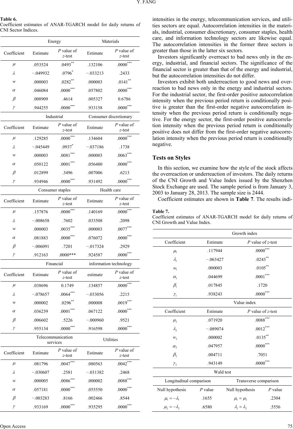
cate that regardless of the style of the stock, investors signifi-
cantly underreact to good news and overreact to bad news, but
volatilities do not present a significant asymmetric pattern.
overreaction or underreaction in the Chinese stock market.
The results of empirical tests based on daily returns indicate
that when the return at time t − 1 is conditionally positive, the
return at time t would present a significant positive first-order
autocorrelation. Moreover, when the return at time t − 1 is con-
ditionally negative, the return at time t would present a signifi-
cant negative first-order autocorrelation. From the behavioral
point of view, investors underreact to good news and overreact
to bad news.
A significant difference in autocorrelation intensity was not
observed in both longitudinal and transverse comparisons.
Tests on Market Cycle
In this section, we examine how the market cycle affects the
overreaction or underreaction of investors. The daily returns of
the Shanghai Composite Index are used. The bull market sam-
ple period is from August 7, 2006 to October 16, 2007. The
sample size is 289. In this period of 14 months, the Shanghai
Composite Index rose from 1547 points to 6992 points, or
293.69%. The bear market sample period is from June 13, 2001
to June 3, 2005. The sample size is 957. In this period of 48
months, the Shanghai Composite Index fell from 2242 points to
1014 points, or 293.69%.
We then conduct a series of robust tests on the underreaction
or overreaction of investors with regard to run length, abnor-
mality degree, time scale, size, sector, style, and market cycle.
Wald coefficients tests are used to compare the autocorrelation
intensities.
The empirical results in this paper could provide significant
reference for investors to adopt a suitable investment strategy.
Acknowledgments
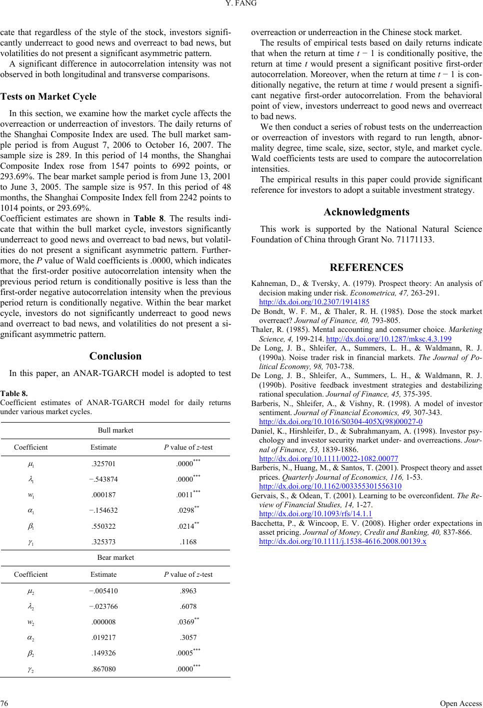
Coefficient estimates are shown in Table 8. The results indi-
cate that within the bull market cycle, investors significantly
underreact to good news and overreact to bad news, but volatil-
ities do not present a significant asymmetric pattern. Further-
more, the P value of Wald coefficients is .0000, which indicates
that the first-order positive autocorrelation intensity when the
previous period return is conditionally positive is less than the
first-order negative autocorrelation intensity when the previous
period return is conditionally negative. Within the bear market
cycle, investors do not significantly underreact to good news
and overreact to bad news, and volatilities do not present a si-
gnificant asymmetric pattern.
This work is supported by the National Natural Science
Foundation of China through Grant No. 71171133.
REFERENCES
Kahneman, D., & Tversky, A. (1979). Prospect theory: An analysis of
decision making under risk. Econometrica, 47, 263-291.
http://dx.doi.org/10.2307/1914185
De Bondt, W. F. M., & Thaler, R. H. (1985). Dose the stock market
overreact? Journal of Finance, 40, 793-805.
Thaler, R. (1985). Mental accounting and consumer choice. Marketing
Science, 4, 199-214. http://dx.doi.org/10.1287/mksc.4.3.199
De Long, J. B., Shleifer, A., Summers, L. H., & Waldmann, R. J.
(1990a). Noise trader risk in financial markets. The Journal of Po-
litical Economy, 98, 703-738.
Conclusion
In this paper, an ANAR-TGARCH model is adopted to test De Long, J. B., Shleifer, A., Summers, L. H., & Waldmann, R. J.
(1990b). Positive feedback investment strategies and destabilizing
rational speculation. Journal of Finance, 45, 375-395.
Table 8.
Coefficient estimates of ANAR-TGARCH model for daily returns
under various market cycles.
Bull market
Coefficient Estimate P value of z-test
1

.325701 .0000***
1

−.543874 .0000***
1
w .000187 .0011***
1

−.154632 .0298**
1

.550322 .0214**
1

.325373 .1168
Bear market
Coefficient Estimate P value of z-test
2

−.005410 .8963
2

−.023766 .6078
2
w .000008 .0369**
2

.019217 .3057
2

.149326 .0005***
2

.867080 .0000***
Barberis, N., Shleifer, A., & Vishny, R. (1998). A model of investor
sentiment. Journal of Financial Economics, 49, 307-343.
http://dx.doi.org/10.1016/S0304-405X(98)00027-0
Daniel, K., Hirshleifer, D., & Subrahmanyam, A. (1998). Investor psy-
chology and investor security market under- and overreactions. Jour-
nal of Finance, 53, 1839-1886.
http://dx.doi.org/10.1111/0022-1082.00077
Barberis, N., Huang, M., & Santos, T. (2001). Prospect theory and asset
prices. Quarterly Journal of Economics, 116, 1-53.
http://dx.doi.org/10.1162/003355301556310
Gervais, S., & Odean, T. (2001). Learning to be overconfident. The Re-
view of Financial Studies, 14, 1-27.
http://dx.doi.org/10.1093/rfs/14.1.1
Bacchetta, P., & Wincoop, E. V. (2008). Higher order expectations in
asset pricing. Journal of Money , Credit and Banking, 40, 837-866.
http://dx.doi.org/10.1111/j.1538-4616.2008.00139.x