Energy and Power Engineering, 2013, 5, 630-635
doi:10.4236/epe.2013.54B122 Published Online July 2013 (http://www.scirp.org/journal/epe)
Rolling Generation Dispatch Based on Ultra-short-term
Wind Power Forecast
Qiushi Xu, Changhong Deng
School of Electrical Engineering, Wuhan University, Wuhan, China
Received January, 2013
ABSTRACT
The power systems economic and safety operation considering large-scale wind power penetration are now facing great
challenges, which are based on reliable power supply and predictable load demands in the past. A rolling generation
dispatch model based on ultra-short-term wind power forecast was proposed. In generation dispatch process, the model
rolling corrects not only the conventional units power output but also the power from wind farm, simultaneously. Sec-
ond order Markov chain model was utilized to modify wind power prediction error state (WPPES) and upd ate forecast
results of wind power over the remaining dispatch periods. The prime-dual affine scaling interior point method was
used to solve the proposed model that taken into account the constraints of multi-periods power balance, unit output
adjustment, up spinning reserve and down spinning reserve.
Keywords: Wind Power Generation; Power System; Rolling Generation Dispatc h; Ultra-short-term Forecast; Markov
Chain Model; Prime-dual Affine Scaling Interior Point Method
1. Introduction
With the shortage of energy worldwide and the environ-
mental concerns of the public, researchers are working
on integrating effectively renewable resources in existing
power grids [1]. As the most promising renewable power
in technology and economy currently, wind power gen-
eration has gradually become a major alternative form.
However, wind energy is non stationary and uncontrolla-
ble, that result in the uncertainty and intermittence of
wind power output and more difficulties to forecast.
Therefore, electric power systems economic and safety
operation considering large-scale wind power penetration
are now facing great challenges, which are based on re-
liable power supply and predictable load demands in the
past.
Advanced power system dispatch technology [2-4] is
one of keys for reducing the impacts of the intermittent
and uncertainty of w ind power outpu t.Economic dispatch
(ED) is a method to schedule the generator outputs with
the predicted load demands over a certain period of time
so as to operate an electric power system most economi-
cally[5].The classical ED problem involved only conven-
tional thermal energy power generators. From the recent
investigations, security economic dispatch in wind power
integrated systems using a conditional risk method was
introduced in article[6], a dynamic economic dispatch
model based on stochastic programming was introduced
in paper[7], optimizing economic/en vironmental d ispatch
with wind and thermal units was introduced in paper[8].
These researches basically concentrated in dealing with
the scheduling and un it commitment problem day-ah ead.
However, the characteristic of the predicting accuracy of
wind power that decreases with the lapse of time will
seriously impair the reasonableness of day-ahead sched-
uling, and bring about heavy burden for regulation ser-
vices which are provided by automatic generation con trol
(AGC). It is necessary to consider linking up day-ahead
scheduling and AGC on the time scale by more meticu-
lous generation diapatch modes. To achieve this we must
incorporate the latest predictive information of wind
power into the generation dispatch process.
The objective of this paper is to incorporate ultra-
short-term wind power predictive information into the
classical economic dispatch problem and propose a roll-
ing generation dispatch mode. In Section II, a method,
which is based on the use of discrete time Markov chain
models of second order, will be utilized to modify the
wind power prediction error state (WPPES) and update
forecast results of wind power over the remaining peri-
ods. Section III will discuss the system power balance
rolling constraints in each dispatch period. Afterward, a
rolling generation dispatch model based on ultra-short-
term wind power forecast is proposed, which rolling cor-
rect not only the conv entional units power output but also
the power from the wind farm, simultaneously. In Sec-

Q. S. XU, C. H. DENG 631
tion IV, the prime-dual affine scaling interior point me-
thod was used to solv e th e p ropo sed mod el. In Section V,
the simulation of the ten-unit test system demonstrates
the economy and effectiveness of the proposed method.
Finally, in Section VI, conclusions are drawn.
2. Wind Power Ultra-short-term Forecast
2.1. Markov Chain Transition Matrices
Estimation of WPPES
Non parametric discrete time Markov Chain models have
been largely used for generating synthetic wind speed
and wind power time series [9-10], providing simulation
results that usually offer excellent fit for both the prob-
ability density function and the autocorrelation function
of the generat ed wind power time series.
In this paper, in order to avoid the cumulative error
form wind forecast to wind power, transition matrices of
WPPES are directly estimated using second order Markov
model as follows:



1
1
W1 WW1W1
W1 WW1
Pr()(),(),,( )
Pr()( ),()
kk
kk
hjhi hi
hjhi hi 
1
i
P
tS PtSPtSPtS
PtSPtSPtS





 

(1)
for each , where is
the prediction erro r state over the time interval

12
,,,,1,,
h
ji iiN

W() h
Pt


1, h
t
h
.
The state variable is discretized defining a finite set of
(representative) values , where N is a ca-
libration parameter, whose setting can refer paper[15].
The minimum and maximum values, 1 and
t

12
,SS

,
N
S
S
N
S
re Pvalu
are
set to W,n and W,n , respectively, wheW,n is
the nominal wind farm power. The remaining
12
,
P P
,es ,SS
N
S are set to the centers of N-2 classes of
equal length defined on the inte

rval

0,1 . In a discrete
finite Markov process,the probability of a state at any
step only depends on t he pre vious state[11] .
For N states, the transition matrix,, is an
matrix. The generic element,, repre-
sents the probability that the state of process at
P( )
h
t(
kij h
ptNNN )
1h
t

is
j
S. An estimate for can be obtained as: ()
kij h
pt
 
 
1
,, ,1,
N
kij h
kij hkij h
j
kij h
j
nt
ptkijptki
nt 
 


(2)
where indicates the number of transitions from
state to state

kij h
nt
,
ki
SS
j
S observed in the sequence of
WPPES dat a .
2.2. Forcecasing Procedure in Generation
Dispatch
The WPPES time series,

W, of a wind farm
must be s established on the basis of historical wind
power data beforehand by
WWW
() ()
hh
h
t
PtPt P


 (3)
where
W average power generated by the wind farm
over ()
h
Pt


1, h
t

Ph
W
t;
h
t

day-ahead forecast power from the wind farm
over


1, hh
tt
.
Indicating with ()
h
t

the state probabilities vector at
time :
h
t


12
()(),(), ,()
hhhN
tttt  h
(4)
whose generic i-th element, ()
ih
t

, represents the prob-
ability that W()
h
Pt

at the time h t equals i. It is
possible to obtain the state probabilities vector at time
, as follows:
S
h
t


-1 2
()( ),()P()
hhh
ttt 

h t (5)
The ultra-short-term wind power forecast procedure
can be defined by (5) and


0-1 02
(),()
hh
tt 

t, the ob-
served state probability vectors at time -1h and -2h,
which are computed utilizing only the most recent data
collected in the time window. Bye modifying the WPPES
over the remaining dispatch periods utilizing the maxi-
mum probability state, future wind power can be rolling
updated.
t
3. Rolling Generation Dispatch M odel
In general situation, day-ahead dispatch is divided into
contiguous and equispaced intervals of length=t

, totally 96 periods a day. Wind power fast fluctua-
tions, especially minute-to-minute variations, are mostly
smoothed by units’ inertia and control dead zones [12],
so it can be con cluded that no t all of wind p ower fluctua-
tions will impair the reasonableness of day-ahead sched-
uling. In order to link up rolling dispatch and day-ahead
scheduling., the time axis is also div ided into intervals of
length
15min
=15 mint

, updating wind power predictive val-
ues and rolling correct units power output and the power
from the wind farm every 15 min.
3.1. Power Balance Rolling Constraints
At the initial time in dispatch period h, system power
balance rolling constraints are established as:
10,
for each0,1,,96, ,1,,96
G
i
Nhh latest
Gt WtLt
i
PPP
hthh


 



(6)
where
G
- h -th dispatch period;
N
h- number of conve ntio nal po wer ge nerat ors;

()
h
Pt
i
Gt
Ph

- power from the i-th conventional generator in

Q. S. XU, C. H. DENG
632
period t after h times corrected. When h equals to 0, it
represents day-ahead schedule power output;
h
Wt
P power from the wind farm in period t after h
times corrected. When h equals to 0, it represents
day-ahead forecast power output from the wind farm;
latest
Lt
P the latest forecast system load in period t.
3.2. Cost Function for Conventional Generator
For the conventional generators, a quadratic cost function
will be assumed, which is practical for most of the cases.
The total operating cost over the remaining dispatch pe-
riods h to 96, , are expressed as:
1(
i
h
Gt
fP
)
)
i
h

)
h

)
96
11
() (
G
i
N
h
Gti Gt
ith
fP CP


 (7)
where i indicates operating cost of i-th conventional
generator, which can be repre sented by
C
2
()
iii
hhh
iGtiGtiGt i
CPaPbPc

 (8)
where i, i and i
c are cost coefficients for the i-th
conventional generator, which are found from the in-
put–output curves of the generators and are dependent on
the particular type of fuel used [13].
a b
3.3. Abandoned Wind Power Calculate
Based on the ultra-short-term wind power forecast values,
abandoned wind power over the remaining dispatch pe-
riods can be calculated as follows:
*
2() (
T
hh
WtWt Wt
th
fPP P



 (9)
where
2(
h
Wt
f
P abandoned wind power over the periods h
to96; *h
Wt
P ultra-short-term forecast power output from the
wind farm in period t.
3.4. Other Constraints
1) Wind farm output limits:
*
0, for each ,1,96
hh
Wt Wt
PP thh

  (10)
2) Generator ramp rate limits:
151 15
iiii
hh
GdnGt GtGup
PTPP PT

  (11)
where i
Gup and i Gdn are ramp-up and ramp-
down rate limits of i-th generator, respectively.
.
P P 
15 =T
15min
3) Generator power operating limits:
min max
iii
h
GGtG
PPP

 (12)
where max
i
G and min
i
G are the minimum and the
maximum powe r ou tputs of i-th generator, respectively.
P P
4) Regulation deviation limits:
In order to ensure the relevance of day-ahead sched-
uleing and rolling scheduleing,the maximum regulation
deviation for conventional generators are set as:
0
ii
h
GtGti
PP



 (13)
where i

is the maximum regulation deviation allow-
able for i-th generators.
5) Up and down spinning reserve constraints:
Integrated large-scale wind power, the system needs
additional spinning reserve capacity to reduce the prob-
ability of load shedding and release regulation capability
of AGC generators.
*
uu
1
%%
G
i
N
latest hh
us
L
tWt
i
PLPw P
Gt



 
 (14)
*
dd
1
%%
G
i
N
latest hh
ds,
L
tWt
i
PLPwP



Gt
i

i
(15)
us ,max10
=min(, )
iii
hh
GtG GtGup
PPPTP

 (16)
ds ,min10
=min( , )
iii
hh
GtGt GGdn
PPPTP

 (17)
where
us ,
iup spinning reserve capacity of i-th generator in
period t;
hGt
P
us ,
i down spinning reserve capacity of i-th genera-
tor in period t ;
hGt
P
10
T%L response time of spinning reserve , ;
10 =10minT
u coefficient of up spinning reserve demand for
system load prediction error;
d coefficient of down spinning reserve demand
for system load prediction error;
%L
u coefficient of up spinning reserve demand for
wind pow er pre d i c t i o n e rror;
%w
d coefficient of down spinning reserve demand
for win d p ower pr ediction e rror.
%w
3.5. Rolling Generation Dispatch Model
The penalty factor,

, is incorporate into rolling gen-
eration dispatch model for coordinating the contradictory
relations between minimizing operating cost of conven-
tional generators and not abandoning wind power .I n this
paper,

is set at a value more than equivalent cost for
converting per unit of wind power into conventional ge-
nerator output, taking value max
i
iiiGi
in the numerical example. Based on (6)-(17) the rolling
generation dispatch model can be written as follows:
max( 2)aaPb  
Minimize
T
12
1
2
Fff  xHxcx
T
(18)
subject to
() hx0 (19)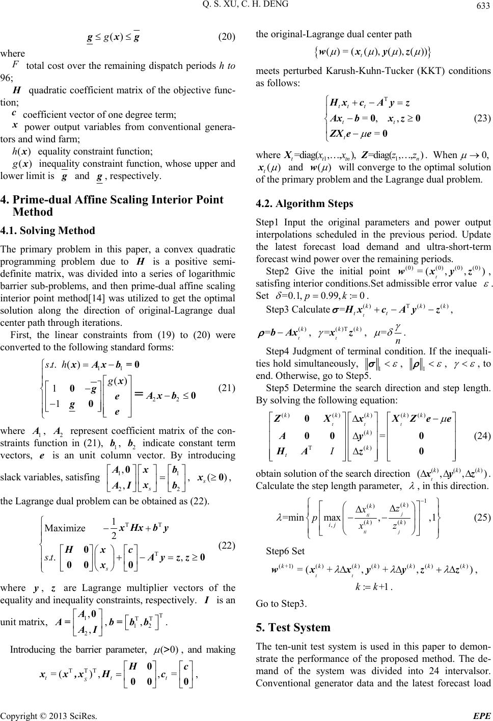

Q. S. XU, C. H. DENG 633
()g
g
x
g
(20)
where
F total cost over the remaining dispatch periods h to
96;
H
quadratic coefficient matrix of the objective func-
tion;
c coefficient vector of one degree term;
x power output variables from conventional genera-
tors and wind farm ;
()hx
()gx equality constraint function; inequality constraint function, whose upper and
lower limit is g and g, respectively.
4. Prime-dual Affine Scaling Interior Point
Method
4.1. Solving Method
The primary problem in this paper, a convex quadratic
programming problem due to
H
is a positive semi-
definite matrix, was divided into a series of logarithmic
barrier sub-problems, and then prime-dual affine scaling
interior point method[14] was utilized to get the optimal
solution along the direction of original-Lagrange dual
center path through iterations.
First, the linear constraints from (19) to (20) were
converted to the following standard forms:
11
22
.. ()
()
1
1
sth
g





 








xAxb=
x
gAx b
e
ge
=
0
00
0
(21)
where 1, 2 represent coefficient matrix of the con-
straints function in (21), 1, 2 indicate constant term
vectors, is an unit column vector. By introducing
A
e
Ab b
slack variables, satisfing , ,
1
22
,
,s
 

 


Ab x
x
AI b
01


()
sx0
the Lagrange dual problem can be obtained as (22).
TT
T
1
Maximize 2
.. ,
s
st




 
 

 
 


xHxby
x Hc
Ay zz
x
00
00 0
(22)
where , y
z
are Lagrange multiplier vectors of the
equality and inequality constraints, respectively. is an I
unit matrix, ,
1
2
,
,



A
A= AI
0T
TT
12
,




b= bb.
Introducing the barrier parameter, (0)

>, and making
TTT
=(),,=
S
ttt



the original-Lagrange dual center path


()=( (),(),())
t

 wxyz
meets perturbed Karush-Kuhn-Tucker (KKT) conditions
as follows:
T
=,,
=
tt t
tt
t








H
xcAyz
Axbx z
ZX ee
0 0
0
(23)
where n1
=diag( ,,),
ttt
x
xX 1. When =diag( ,,)
n
zzZ0,


t()

x and ()

w will converge to the opti mal solution
of the primary problem and the Lagrange dual problem.
4.2. Algorithm Steps
Step1 Input the original parameters and power output
interpolations scheduled in the previous period. Update
the latest forecast load demand and ultra-short-term
forecast wind po w er ove r the remaining periods.
Step2 Give the initial point t
(0)(0)(0) (0)
=(,,)wx
y
z,
satisfing interior conditions.Set admissible er ror value

.
Set =0.1,0.99,: 0pk



()
.
Step3 CalculateT ()()kkk
=t
tt
 
H
xcA
y
z 
()T ()
t
kk
xz
,
, ,
()
=t
k
bAx  =  =n


 .
Step4 Judgment of terminal condition. If the inequali-
ties hold simultaneously, 1

  , 1

  ,



, to
end. Otherwise, go to Step5.
Step5 Determine the search direction and step length.
By solving the following equation:
()()()() ()
()
T()
=
tt t
kkkkk
k
k
tI


 


 


 

 


 

 
ZXxXZe
Ay
HA z
0
00 0
0
e
)
(24)
obtain solution of the search directio n t
()()()
(,,
kkk
x
y
z.
Calculate the step length parameter,

, in this direction.
1
()
()
() ()
,
=min max,,1
j
ti
ti j
k
k
kk
ij
z
x
pxz






















(25)
Step6 Set
(+1)()()()() ()()
=( +,+,)
tt
kkkkkk
 wxxyyzz
:+ 1 kk
k
,

.
Go to Step3.
5. Test System
The ten-unit test system is used in this paper to demon-
strate the performance of the proposed method. The de-
mand of the system was divided into 24 intervalsor.
Conventional generator data and the latest forecast load





H
c
xx,xH c
0
00 0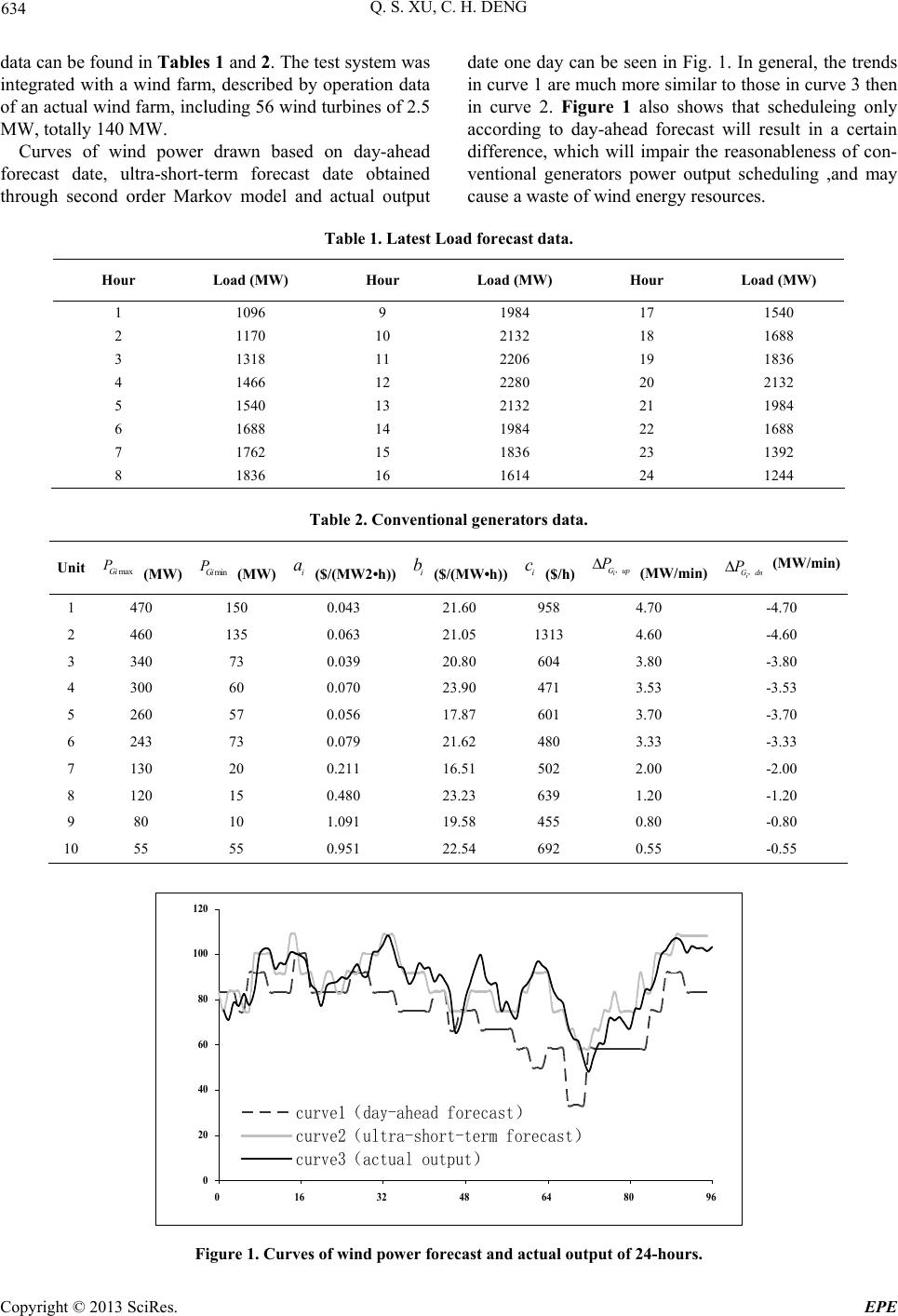
,

Q. S. XU, C. H. DENG
634
data can be found in Ta ble s 1 an d 2. The test system was
integrated with a wind farm, described by operation data
of an actual wind farm, including 56 wind turbines of 2.5
MW, totally 140 MW.
Curves of wind power drawn based on day-ahead
forecast date, ultra-short-term forecast date obtained
through second order Markov model and actual output
date one day can be seen in Fig. 1. In general, the trends
in curve 1 are much more similar to those in curve 3 then
in curve 2. Figure 1 also shows that scheduleing only
according to day-ahead forecast will result in a certain
difference, which will impair the reasonableness of con-
ventional generators power output scheduling ,and may
cause a waste of wind energy resources.
Table 1. Latest Load forecast data.
Hour Load (MW) Hour Load (MW) Hour Load (MW)
1 1096 9 1984 17 1540
2 1170 10 2132 18 1688
3 1318 11 2206 19 1836
4 1466 12 2280 20 2132
5 1540 13 2132 21 1984
6 1688 14 1984 22 1688
7 1762 15 1836 23 1392
8 1836 16 1614 24 1244
Table 2. Conventional generators data.
Unit maxGi
P (MW) minGi P (MW) i a ($/(MW2•h))i b ($/(MW•h))i c ($/h)i
Gup
P

， (MW/min) i
Gdn
P， (MW/min)
1 470 150 0.043 21.60 958 4.70 -4.70
2 460 135 0.063 21.05 1313 4.60 -4.60
3 340 73 0.039 20.80 604 3.80 -3.80
4 300 60 0.070 23.90 471 3.53 -3.53
5 260 57 0.056 17.87 601 3.70 -3.70
6 243 73 0.079 21.62 480 3.33 -3.33
7 130 20 0.211 16.51 502 2.00 -2.00
8 120 15 0.480 23.23 639 1.20 -1.20
9 80 10 1.091 19.58 455 0.80 -0.80
10 55 55 0.951 22.54 692 0.55 -0.55
0
20
40
60
80
100
120
0 163248648096
curve1（day-ahead forecast）
curve2（ultra-short-term forecast）
curve3（actual output）
Figure 1. Curves of wind power forecast and actual output of 24-hours.

Q. S. XU, C. H. DENG 635
Table 3. The comparative of objective function values.
Correction Average abandoned wind power (MW) Cost for conventional generators ($) Total cost ($)
before 17.5379 5016455 5076029
after 2.3008 4945263 4953078
Rolling dispatch algorithm is performed at period 30
when day-ahead forecast appears larger deviation shown
in Figure 1. The hardware environment for testing are
4GB memory and Intel(R)/Core(TM)2/Duo CPU2.80Ghz,
programming in MATLAB. In the example, 0.1
i


,
, , u, du %0.1wd%0.3w%0.05L%0.05L

,
202.8

, 0.01

. In this case, the computation time
is 1.94s and iteration times are 14, that can meet the
needs of online rolling generation dispatch computing.
The objective function values before and after correction
are shown in Table 3, which shows that after rolling
correction average abandoned wind power per one pe-
riod has reduced 15.2371 MW and operating cost for
conventional generators has been saved 71192 $. Thus,
rolling generation dispatch can not only reduce aban-
doned wind power, but also make the power system
economizing in energy consumption with more wind
power accommodated.
6. Conclusions
In this paper, a rolling generation dispatch model based
on ultra-short-term wind power forecast, utilizing Markov
chain model method, was proposed. In generation dis-
patch process, the model rolling correct not only the
convention al units power output but also the power from
wind farm, simultaneously. The simulation results illus-
trates that the model can effectively promote power sys-
tem accommodating wind power and optimizing the op-
eration cost. Rolling generation dispatch is necessary in
the background of the rapid development of wind power,
energy conservation and emission reduction.
REFERENCES
[1] European Smart Grid Technology Platform, “Vision and
Strategy for Europe’s Electricity Networks of the Future,”
EU Commission, Directorate-General for Research, In-
formation and Communication Unit, Brussel, Belgium,
2006.
[2] T. Y. Lee, “Optimal Spinning Reserve for a
Wind-Thermal Power System Using EIPSO,” IEEE
Transacti Power Systems, Vol. 22, 2007, pp. 1612-1621.
doi:10.1109/TPWRS.2007.907519
[3] J. Hetzer and D. C. Yu, “An Economic Dispatch Model
Incorporating Wind Power,” Journal of IEEE Trans. En-
ergy Conversion, Vol. 23, 2008, pp. 603-611.
doi:10.1109/TEC.2007.914171
[4] H. Siahkali and M. Vakilian, “Stochastic Unit Commit-
ment of Wind Farms Integrated in Power System,” Elec-
tric Power Systems Research, Vol. 80, 2010, pp.
1006-1017. doi:10.1016/j.epsr.2010.01.003
[5] A. J. Wood and B. F. Wollenberg, Power Generation
Operation and Con-trol, 2nd ed, New York, Wiley, 1996.
[6] R. J. Zhou, L. H. Yao, et al., “Security Economic Dis-
patch in Wind Power Integrated Systems Using a Condi-
tional Risk Method,” Proceedings of the CSEE, Vol. 32,
2011, pp. 56-63.
[7] Y. Z. Sun, J. Wu, G.J. Li and J. He, “Dynamic Economic
Dispatch Considering Wind Power Penetraion Based on
Wind Speed Forecasting and Stochastic Programming,”
Proceedings of the CSEE, Vol. 29, 2009, pp. 41-47.
[8] W. Qiu, J. H. Zhang and N. Liu, “Model and Solution for
Environmental/Economic Dispatch Considering
Large-Scale Wind Power Penetration,” Proceedings of
the CSEE, Vol. 7, 2011, pp. 8-16.
[9] K. Brokish and J. Kirtley, “Pitfalls of Modeling Wind
Power Using Markov Chains,” in Power Systems Con-
ference and Exposition, PSCE’09, IEEE/PES, 2009, pp.
1-6.
[10] A. Shamshad, M. A. Bawadi, W. M. A. Wan Hussin, T. A.
Majid and S. A. M. Sanusi, “First and Second Order
Markov Chain Models Forsynthetic Generation of Wind
Speed Time Series,” Energy, Vol. 30, No. 5, 2005, pp.
693-708.
[11] J. G. Kemeny and J. L. Snell, “Finite Markov Chains,”
2nd edition, Springer, New York, 1976.
[12] H. Banakar, C. Luo and B. K. Ooi, “Impacts of Wind
Powerminute-to-minute Variations on Power System Op-
eration,” IEEE Transacti on Power Systems, Vol. 23,
2008, pp. 150-160. doi:10.1109/TPWRS.2007.913298
[13] A. J. Wood and B. F. Wollenberg, “Power Generation,
Operation and Control,” 2nd edition, Wiley, New York,
1996.
[14] H. Wei, H. Sasaki and R. Yokoyama, “An Application of
Interior Pointquadratic Programming Algorithm to Power
System Optimization Problems,” IEEE Transacti on
Power Systems, Vol. 11, No. 1, 1996.