Energy and Power Engineering, 2013, 5, 493-497
doi:10.4236/epe.2013.54B095 Published Online July 2013 (http://www.scirp.org/journal/epe)
Fast Algorithm for Prediction of Airfoil Anti-icing
Heat Load*
Xueqin Bu, Rui Yang, Jia Yu, Xiaobin Shen, Guiping Lin
School of Aeronautic Science and Engineering, Beihang University, Beijing, China
Received January, 2013
ABSTRACT
Many flight and icing conditions should be considered in order to design an efficient ice protection system to prevent
ice accretion on the aircraft surface. The anti-icing heat load is the basic knowledge for the design of a thermal an-
ti-icing system. In order to help the design of the thermal anti-icing system and save the design time, a fast and effi-
ciency method for prediction the anti-icing heat load is investigated. The computation fluid dynamics (CFD) solver and
the Messinger model are applied to obtain the snapshots. Examples for the calculation of the anti-icing heat load using
the proper orthogonal decomposition (POD) method are presented and compared with the CFD simulation results. It is
shown that the heat loads predicted by POD method are in agreement with the CFD computation results. Moreover, it is
obviously to see that the POD method is time-saving and can meet the requirement of real-time prediction.
Keywords: Anti-icing; Heat Load; Proper Orthogonal Decomposition
1. Introduction
Aircraft icing is a thermodynamic phenomenon that leads
to the formation of ice on aircraft in flight. Severe in-
flight icing is a serious hazard that destroys the clean
aerodynamic shape of the airfoil, resulting in increased
drag, decreased lift, reduced aircraft stability, perform-
ance and controllability. Thermal anti-icing system, used
as the most popular means of ice prevention in icing
conditions, operates to keep the surface temperature and
the water collected by the aircraft above the freezing
point.
During the process of the design of the anti-icing sys-
tem, many flight and icing conditions should be consid-
ered for the calculation of the water droplet impingement
and the anti-icing heat load to have knowledge of how
about the most severe condition and how much heat flux
should be supplied for anti-icing. Generally, the CFD
method is used for the air flow simulation around the
object and then the thermal analysis are applied to calcu-
late the heat load [1] considering the whole flight and
icing conditions under FAR 25 Appendix C. This would
lead to very large computation work and expend much
computation time. In order to help the design and save
the design time, a fast and efficiency method for predic-
tion the anti-icing heat load is investigated in this paper.
The proper orthogonal decomposition (POD) [2] tech-
nique is a powerful reduced-order model (ROM), which
can effectively reduce the degree of freedom for physical
problems with high precision, thus reducing the calcula-
tion time and saving the data storage significantly. POD
has been used extensively in the field of flow and heat
transfer computation [3,4] to predict these problems ac-
curately in very short time.
In this paper the CFD method is used to obtain the
snapshots (samples) for the POD analysis. The POD me-
thod is studied and used for the fast prediction of the heat
loads. The effects of the variables for the POD prediction
of the heat load are investigated and the results are com-
pared with the CFD simulation results.
2. POD Methodology
POD method can rapidly reconstruct the flow informa-
tion applying a data set called snapshots or samples of
the physical properties. The essence of the POD method
is the extraction of a set of eigenfunctions which can best
describes the dominant features of the flow or heat trans-
fer. Once these eigenfunctions are calculated, the ap-
proximate states of the flow field and heat transfer pa-
rameters can be obtained by superposition of them.
POD method requires a set of snapshots which can be
obtained either from numerical calculations or tests. In
this paper, the snapshots are obtained from the CFD
analysis. The snapshot i, a vector which describes a
certain physical field, can be any type of the flow vari-
U
*Supported by the National Natural Science Foundation of China
(Grant No. 51206008).

X. Q. BU ET AL.
494
able, such as velocity, pressure, ice shape [5,6], or an-
ti-icing heat load, as in this paper. If each has N
sample values, a set of M snapshots forms a
i
U
NM

matrix , which can be expressed by:
U

1,,M
UU U

. (1)
As mentioned above, POD method presents the main
characteristics of the flow by using a set of eigenfunc-
tions. This means that a set of proper orthogonal decom-
position modes
j

, should be found, and then can
be expressed by:
i
U
,
Mij
j
j=1
 

i
U=

(2)
where i
j

is a set of sample coefficients for the proper
orthogonal decomposition modes
j

, can be calculated
by:
(,)
iji
j
 =U  , (3)
where j denotes the proper orthogonal decomposi-
tion mode, and i denotes the snapshot.
th
j
th
i
All the
j

form the proper orthogonal decomposi-
tion modes matrix

:

1,, M
  

, (4)
where M is the number of snapshots. The matrix

, of
the same dimensionality as U, satisfies the constraint



 . The elements of the modes are defined as:
,UV

 (5)
where is the eigenvector matrix of : V C
,CV V 
(6)
 is a diagonal matrix storing the eigenvalues i

of
the positive definite covariance matrix . The entries of
are defined as:
C
C
1
.
C
Nij
ijk k
k
CUUM

 (7)
Thus, the problem of solving the proper orthogonal
decomposition modes changes into that of solving the
eigenvalues and eigenvectors of the matrix . Obvi-
ously, is a C
M
M matrix, so the matrix to be solved
becomes much smaller, reducing from a size N (the
number of grid points) to a size M (number of snapshots).
This is one of the advantages of using the POD tech-
nique.
After the proper orthogonal decomposition modes
j

and sample coefficients i
j

are obtained from the ma-
trix which can be calculated from the snapshot ma-
trix , the approximate states of the flow field can be
obtained by linear superposition of the proper orthogonal
decomposition modes, shown as follows:
C
U
.
M
p
od j
j
j=1
 

pod
U=

(8)
To predict a field which is not part of the snapshots, an
interpolation method must be employed to obtain the
POD coefficients . The linear interpolation method
is employed to compute the coefficients in this paper.
POD
j

Moreover, the magnitude of each eigenvalue i

de-
termines the energy contained in the corresponding mode.
The ratio of the energy contained in a certain mode can
be measured by:
1
Energy .
i
M
i
i



 (9)
Therefore, if necessary, the modes that contain less
energy can be negligible, resulting in the reduction of
proper orthogonal decomposition modes. The approxi-
mation by POD calculation of the linear combination of
eigenvectors can be written as:
,
l
p
od j
j
j=1
 

pod
U=

(10)
where l is the proper orthogonal decomposition modes
used for the construction of the approximation by POD,
so
M
l. If some proper orthogonal decomposition
modes are ignored, the flow field reconstructed by POD
will be different from that reconstructed by all modes.
The inaccuracy can be controlled by the total energy of
all the used proper orthogonal decomposition modes.
The most time cost during the calculation by POD is
that of solving the eigenvalues and eigenvectors of the
M
M

matrix , and the total calculation process only
takes a few seconds.
C
In this paper, the effectiveness of the POD method in
prediction the anti-icing heat load on an airfoil is inves-
tigated and the effects of the ambient temperature, flight
velocity and liquid water content (LWC) on the POD-
reconstructed anti-icing heat load are studied.
3. Anti-icing Heat Load Prediction for
Snapshots
The prediction of the anti-icing heat load generally has
four steps: 1) air flow field calculation, 2) water droplet
impingement calculation, 3) external convective heat
transfer coefficient prediction, 4) anti-icing heat load
analysis.
In this paper, for the snapshots, the Eulerian method is
used for the calculation of the water droplet impingement.
The boundary layer integrated method is used for the
calculation of the external heat transfer coefficient. The
anti-icing heat loads simulation is based on the Mess-
inger model. The Computational Fluid Dynamic (CFD)
tool Fluent and its User Defined Function (UDF) are ap-
plied to implement the above computations for the snap-
shots. Details about the method and analysis can be

X. Q. BU ET AL. 495
found in Reference [1,7,8] written by authors.
4. POD Validation and Results Analysis
In this paper, the POD method, at first, is applied to the
prediction of anti-icing heat loads for 2D viscous flow
under a one-variable problem, here being ambient tem-
perature. The calculation process of the POD method is
introduced in detail. Then, the anti-icing heat loads pre-
dictions by POD under two-variable and three-variable
problems have been investigated.
An airfoil which has 344 control volumes is taken into
consideration for the study. The anti-icing heat load
samples of each control volume on the airfoil under cer-
tain flight and icing conditions are obtained by the CFD
method. Besides three parameters which are the ambient
temperature, the velocity and the LWC, the other pa-
rameters in all cases are the same, which are: 20μm as
the mean volume diameter, 2° as the angle of attack,
90KPa as the ambient pressure, 25℃ as the surface tem-
perature of the airfoil.
4.1. One Parameter POD Application for Heat
Load
It is well known that the ambient temperature has a great
influence on anti-icing heat loads. Therefore, firstly, the
effect of the ambient temperature on the POD-predicted
anti-icing heat loads on an airfoil is investigated and the
effectiveness of the POD method is studied. In this sec-
tion, the LWC and the flight velocity are 0. 6 g/m3 and
90 m/s individually. The ambient temperature is from -30
to - ℃. The anti-icing heat loads, which are obtained by
CFD method, at the ambient temperature of -30, -25, -20,
-15, -10, -5℃ are taken as samples. So a 344 × 6 matrix
forms and M = 6. The anti-icing heat loads under various
ambient temperatures, predicted by the CFD method, are
shown in Figure 1.
-0.75-0.50-0.250.00 0.25 0.50 0.75
5
10
15
20
25
30
35
40
45
s
(
m
)
Heatload(kW/m
2
)
temp= -5 ℃
temp= -10 ℃
temp= -15 ℃
temp= -20 ℃
temp= -25 ℃
temp= -30 ℃
Figure 1. Anti-icing heat loads at different ambient tempera-
tures (CFD method).
According to the sample matrix , the corresponding
matrix can be calculated using Equation (7), and
is a 6 × 6 matrix because there are 6 snapshots. The re-
sults of matrix are showed in Table 1. Then the or-
dered eigenvectors and eigenvalues of matrix C are
calculated from Equation (6). The eigenvalues are
showed in Table 2.
U
C
C
C
It can be found that the first eigenvalue is much larger
than others from Table 2, which means that the energy
contained in the corresponding mode is very large. It can
be concluded that the first mode is vital to the prediction
and it determines the broad contour of the anti-icing heat
loads distribution.
Next, the ultimately used proper orthogonal decompo-
sition modes can be obtained by orthogonalizing the ma-
trix

, which can be calculated from Equation (5). Here
all the proper orthogonal decomposition modes are used
for calculation. The sample coefficient i

for the cor-
responding proper orthogonal decomposition mode can
be obtained using Equation (3). The results are shown in
Table 3. It is obvious that each sample coefficient for the
first proper orthogonal decomposition mode is much lar-
ger than other modes, indicating that the first mode
makes a significant contribution on the POD calculation.
Table 1. C matrix values.
23720.9322564.5621285.6119996.39 18478.0216893.21
22564.5621468.5120254.5519030.61 17585.8616077.71
21285.6120254.5519118.8117970.34 16609.7215187.40
19996.3919030.6117970.3416898.27 15622.5114285.26
18478.0217585.8616609.7215622.51 14465.4713236.85
Table 2. Eigenvalues.
case Λ
1 107679.734
2 101.829
3 18.207
4 4.686
5 1.147
Table 3. Sample coefficients.
а1 а2 а3 а4 а5 a6
1 269.250294.367318.333 338.661 358.786377.063
2 16.60610.9602.040 -2.865 -8.775-11.213
3 -5.3871.847 6.790 2.931 -1.625-4.414
4 -2.1704.166 -1.467 -1.593 -0.1911.148
5 0.081 -0.2900.805 -0.263 -1.9171.550
6 0.085 -0.1590.861 -1.384 0.593 0.016

X. Q. BU ET AL.
496
After the above calculations, the POD model has been
basically established. The anti-icing heat loads at the
ambient temperature of -23, -12℃ are predicted using
the POD approach. The predicted results are compared
with the results from CFD method. The POD coefficients
are interpolated by the linear method, and the pre-
dicted anti-icing heat loads are calculated using Equation
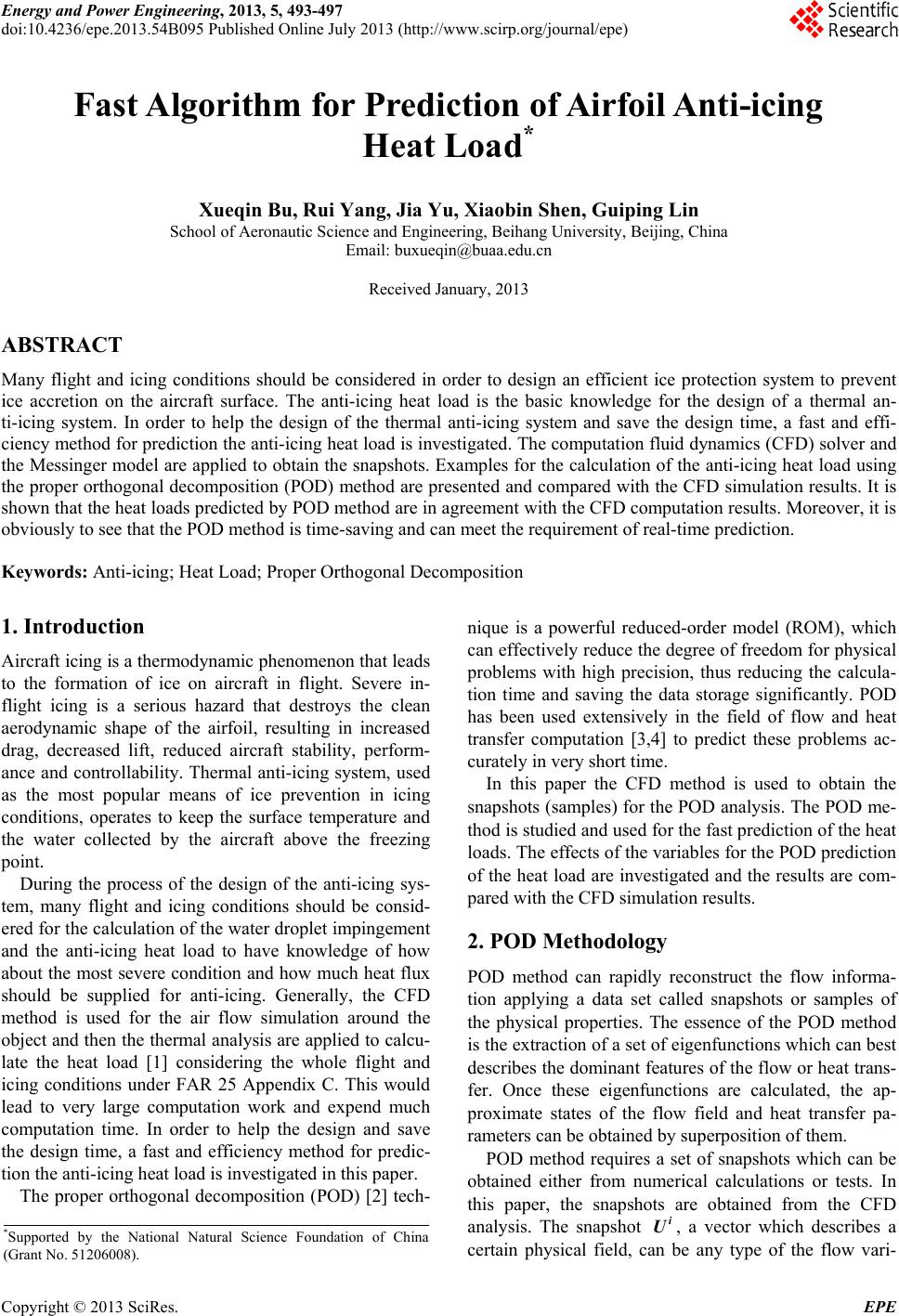
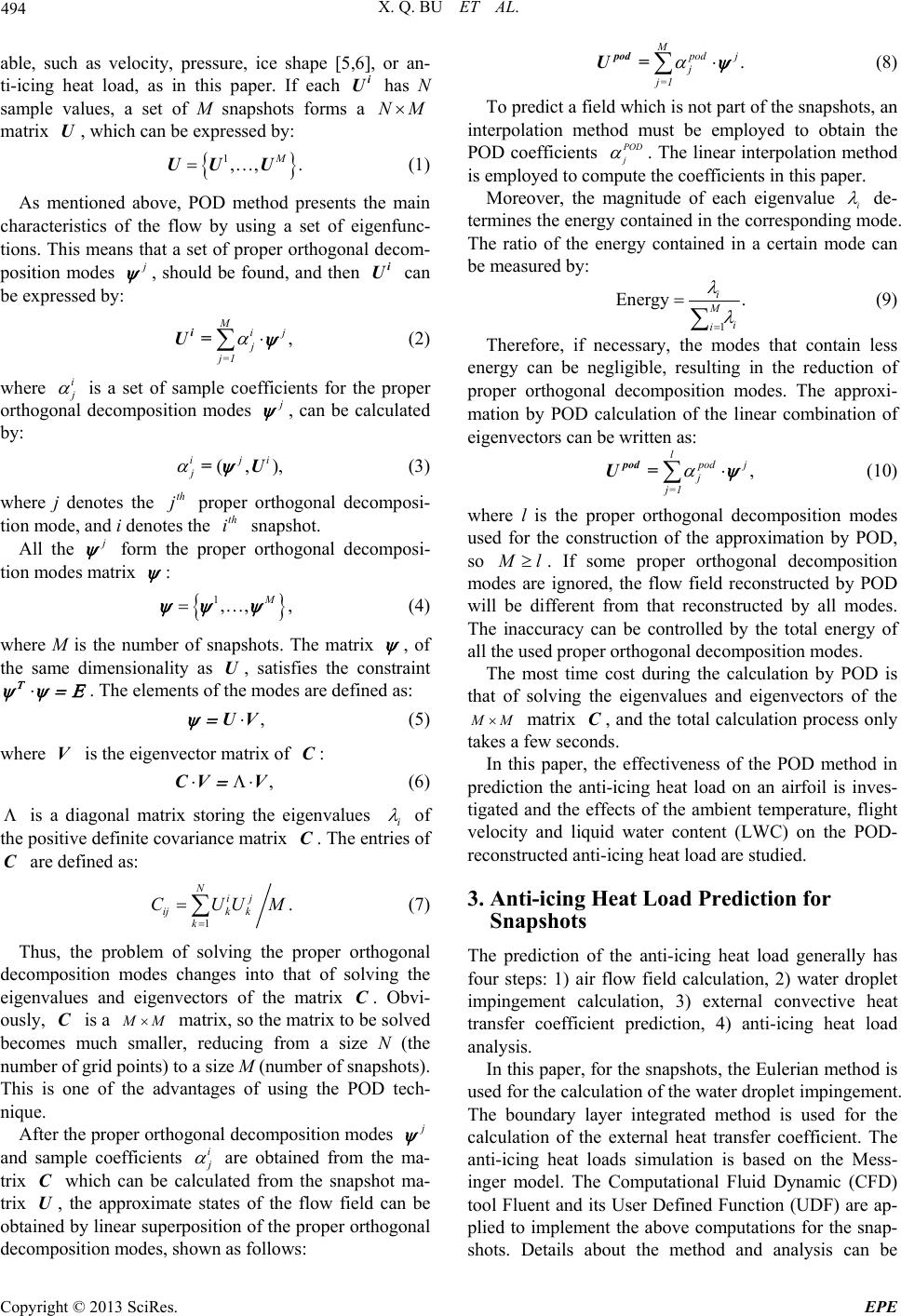
(10). Figure 2 shows the heat loads comparisons be-
tween the POD solutions and the CFD method, which
indicates that the results nearly the same between the
POD and CFD method under the same conditions.
Therefore, the POD method can be applied very well to
predict the heat load when one parameter changes.
POD
j

4.2. Two Parameters POD Application for Heat
Load
In this section, the POD method is used to predict the
anti-icing heat loads under two-variable problem, here
being the ambient temperature and flight velocity. The
LWC is 0.6 g/m3. The samples are obtained at the ambi-
ent temperature of -30, -25, -20, -15, -10, -5 ℃ and the
flight velocity of 90, 100, 110, 120, 130, 140 m/s. Thus
the number of the snapshots is 36.
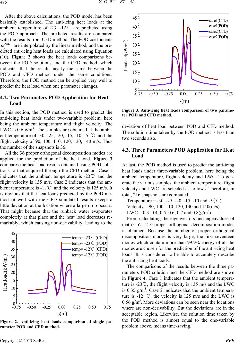
All the 36 proper orthogonal decomposition modes are
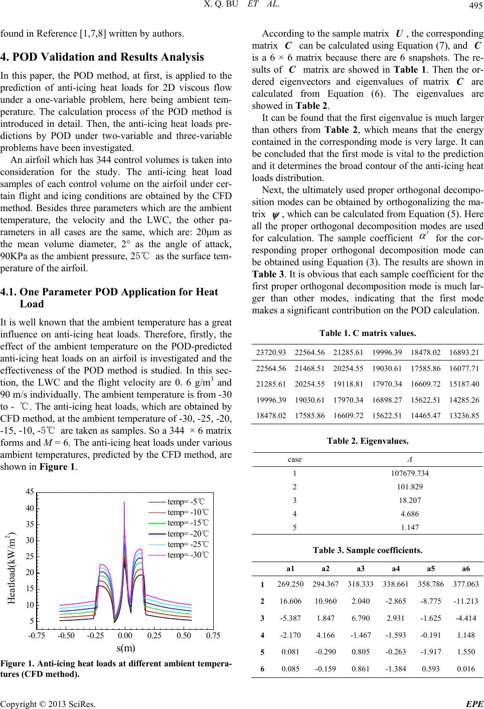
applied for the prediction of the heat load. Figure 3
compares the heat load results obtained using POD solu-
tions to that acquired through the CFD method. Case 1
indicates that the ambient temperature is -23℃ and the
flight velocity is 135 m/s. Case 2 indicates that the am-
bient temperature is -12℃ and the velocity is 125 m/s. It
is obvious that the heat loads predicted by the POD me-
thod fit well with the CFD simulated results except a
little deviation at the location where a large drop occurs.
That might because that the runback water evaporates
completely at that place and the heat load decreases re-
markably, which causing non-derivability, leading to the
-0.75 -0.50 -0.250.000.250.500.75
0
5
10
15
20
25
30
35
40
45
s
(
m
)
Heatload(kW/m
2
)
temp= -23 (CFD) ℃
temp= -23 (POD) ℃
temp= -12 (CFD) ℃
temp= -12 (POD) ℃
Figure 2. Anti-icing heat loads comparison of single pa-
rameter POD and CFD method.
-0.75-0.50-0.250.00 0.25 0.50 0.75
5
10
15
20
25
30
35
40
45
s(m)
Heatload(kW/m
2
)
case1(CFD)
case1(POD)
case2(CFD)
case2(POD)
Figure 3. Anti-icing heat loads comparison of two parame-
ter POD and CFD method.
deviation of heat load between POD and CFD method.
The solution time taken by the POD method is less than
two seconds also.
4.3. Three Parameters POD Application for Heat
Load
At last, the POD method is used to predict the anti-icing
heat loads under three-variable problem, here being the
ambient temperature, flight velocity and LWC. To gen-
erate the various samples, the ambient temperature, flight
velocity and LWC are selected as follows. Therefore, in
total, 216 snapshots are computed.
Temperature = -30, -25, -20, -15, -10 and -5(℃ )
Velocity = 90, 100, 110, 120, 130 and 140(m/s)
LWC = 0.3, 0.4, 0.5, 0.6, 0.7 and 0.8(g/m3)
From calculating the eigenvectors and eigenvalues of
matrix , 216 proper orthogonal decomposition modes
is obtained. Because the number of proper orthogonal
decomposition modes is very large, the first seventeen
modes which contain more than 99.9% energy of all the
modes are chosen for the prediction of the anti-icing heat
loads. It is considered to be able to accurately describe
the anti-icing heat loads.
C
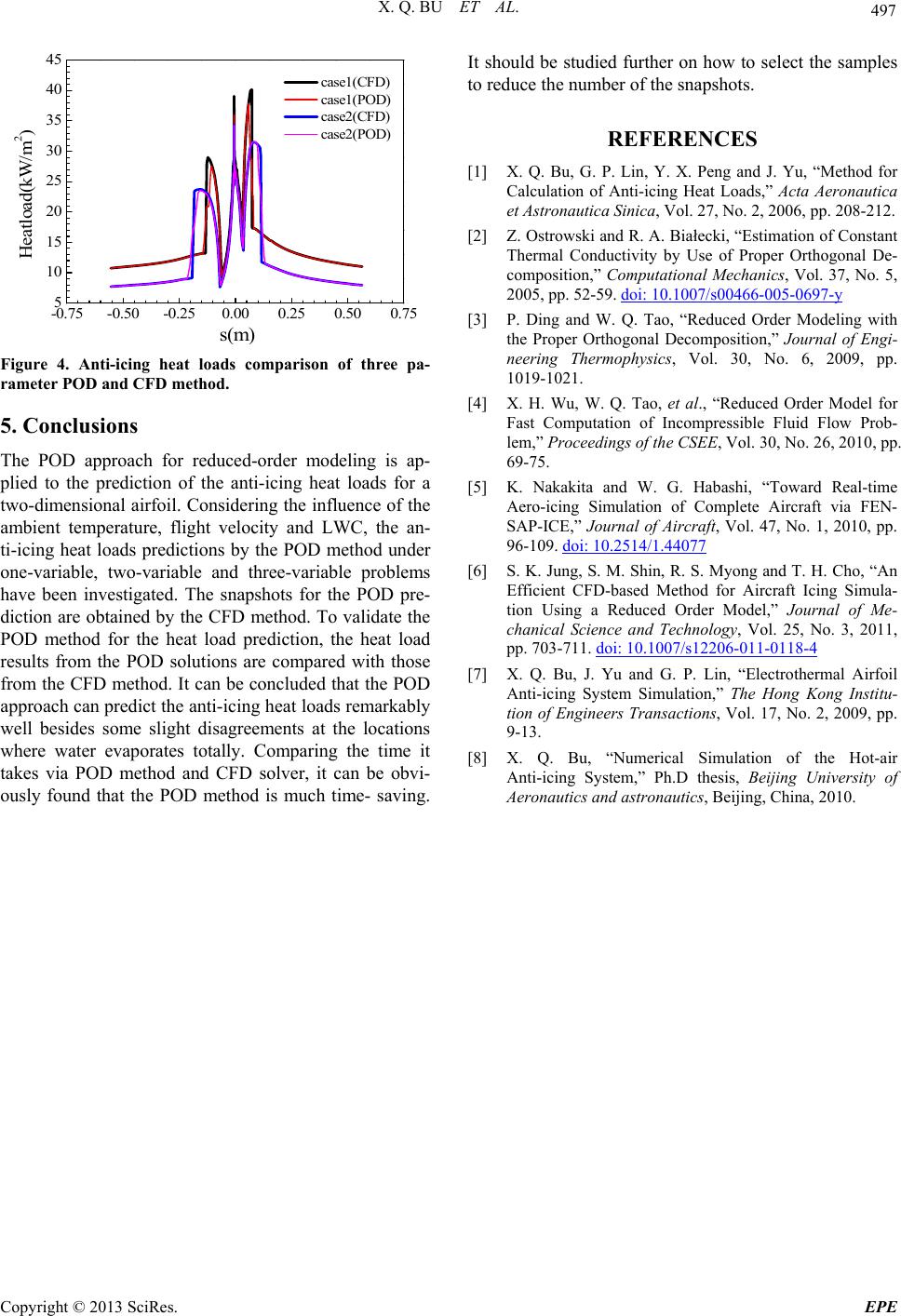
The comparisons of the results between the three pa-
rameters POD solution and the CFD method are shown
in Figure 4. Case 1 indicates that the ambient tempera-
ture is -23℃, the flight velocity is 135 m/s and the LWC
is 0.35 g/m3. Case 2 indicates that the ambient tempera-
ture is -12 ℃, the velocity is 125 m/s and the LWC is
0.56 g/m3. More deviations can be seen near the locations
where are non-derivability. But the deviations are in the
acceptable region. Likewise, the solution time taken by
the POD method is almost equal to the one-variable
problem above, means time-saving.

X. Q. BU ET AL.
497
-0.75-0.50-0.250.00 0.25 0.50 0.75
5
10
15
20
25
30
35
40
45
s
(
m
)
Heatload(kW/m
2
)
case1(CFD)
case1(POD)
case2(CFD)
case2(POD)
Figure 4. Anti-icing heat loads comparison of three pa-
rameter POD and CFD method.
5. Conclusions
The POD approach for reduced-order modeling is ap-
plied to the prediction of the anti-icing heat loads for a
two-dimensional airfoil. Considering the influence of the
ambient temperature, flight velocity and LWC, the an-
ti-icing heat loads predictions by the POD method under
one-variable, two-variable and three-variable problems
have been investigated. The snapshots for the POD pre-
diction are obtained by the CFD method. To validate the
POD method for the heat load prediction, the heat load
results from the POD solutions are compared with those
from the CFD method. It can be concluded that the POD
approach can predict the anti-icing heat loads remarkably
well besides some slight disagreements at the locations
where water evaporates totally. Comparing the time it
takes via POD method and CFD solver, it can be obvi-
ously found that the POD method is much time- saving.
It should be studied further on how to select the samples
to reduce the number of the snapshots.
REFERENCES
[1] X. Q. Bu, G. P. Lin, Y. X. Peng and J. Yu, “Method for
Calculation of Anti-icing Heat Loads,” Acta Aeronautica
et Astronautica Sinica, Vol. 27, No. 2, 2006, pp. 208-212.
[2] Z. Ostrowski and R. A. Białecki, “Estimation of Constant
Thermal Conductivity by Use of Proper Orthogonal De-
composition,” Computational Mechanics, Vol. 37, No. 5,
2005, pp. 52-59. doi: 10.1007/s00466-005-0697-y
[3] P. Ding and W. Q. Tao, “Reduced Order Modeling with
the Proper Orthogonal Decomposition,” Journal of Engi-
neering Thermophysics, Vol. 30, No. 6, 2009, pp.
1019-1021.
[4] X. H. Wu, W. Q. Tao, et al., “Reduced Order Model for
Fast Computation of Incompressible Fluid Flow Prob-
lem,” Proceedings of the CSEE, Vol. 30, No. 26, 2010, pp.
69-75.
[5] K. Nakakita and W. G. Habashi, “Toward Real-time
Aero-icing Simulation of Complete Aircraft via FEN-
SAP-ICE,” Journal of Aircraft, Vol. 47, No. 1, 2010, pp.
96-109. doi: 10.2514/1.44077
[6] S. K. Jung, S. M. Shin, R. S. Myong and T. H. Cho, “An
Efficient CFD-based Method for Aircraft Icing Simula-
tion Using a Reduced Order Model,” Journal of Me-
chanical Science and Technology, Vol. 25, No. 3, 2011,
pp. 703-711. doi: 10.1007/s12206-011-0118-4
[7] X. Q. Bu, J. Yu and G. P. Lin, “Electrothermal Airfoil
Anti-icing System Simulation,” The Hong Kong Institu-
tion of Engineers Transactions, Vol. 17, No. 2, 2009, pp.
9-13.
[8] X. Q. Bu, “Numerical Simulation of the Hot-air
Anti-icing System,” Ph.D thesis, Beijing University of
Aeronautics and astronautics, Beijing, China, 2010.