Journal of Software Engineering and Applications, 2013, 6, 22-29
doi:10.4236/jsea.2013.67B005 Published Online July 2013 (http://www.scirp.org/journal/jsea)
The Constrained Mean-Semivariance Portfolio
Optimization Problem with the Support of a Novel
Multiobjective Evolutionary Algorithm
K. Liagkouras, K. Metaxiotis
DSS Lab., Department of Informatics, University of Piraeus, Piraeus, Greece.
Received May, 2013
ABSTRACT
The paper addresses the constrained mean-semivariance portfolio optimization problem with the support of a novel
multi-objective evolutionary algorithm (n-MOEA). The use of semivariance as the risk quantification measure and the
real world constraints imposed to the model make the problem difficult to be solved with exact methods. Thanks to the
exploratory mechanism, n-MOEA concentrates the search effort where is needed more and provides a well formed effi-
cient frontier with the solutions spread across the whole frontier. We also provide evidence for the robustness of the
produced non-dominated solutions by carrying out, out-of-sample testing during both bull and bear market conditions
on FTSE-100.
Keywords: Multiobjective Optimization; Evolutionary Algorithms; Portfolio Optimization
1. Introduction
Portfolio optimization is the process of choosing the as-
sets and their proportions, so that it is attained the maxi-
mum profitability for the risk undertaken. MOEAs tech-
niques applied to the portfolio selection problem have
become increasingly popular relatively recen tly. Not only
because they provide a fast and reliable way of calculat-
ing computationally demanding financial models but also
why revolutionized the financial modeling research field
itself by developing innovative algorithmic approaches
for solving difficult financial problems that in many cas-
es cannot be solved with exact methods. Over the past
years researchers developed several approaches for the
solution of the portfolio optimization problem with the
use of MOEAs. Most of the early work on MOEAs
adopts the unconstrained Markowitz Mean – Variance
(MV) model [2, 4]. Obvio u sl y , the p rac t i cal usef ul ness of
such a model is limited to acad emic purposes an d cannot
address the complexity and multiple real world con-
straints faced by portfolio managers. More recent studies,
incorporate a number of constrain ts into the optimization
model, but do not examine how these constraints affect
the evolutionary search process and the efficient frontier
formulation. Additionally, still the majority o f the studies
use variance [3] for the quantification of portfolio risk
although it’s well known undesirable mathematical
properties [1].
Our paper proposes a bi-objective return semivariance
portfolio optimization model that incorporates a number
of real world constraints such as cardinality constraints,
floor and ceiling constraints, non-negativity constraint
and budget constraint and analyzes their effects on the
efficient frontier formulation. Finally, we provide em-
pirical evidence for the robustness of the proposed
methodology by performing, out-of-sample experiments
during both bull and bear market conditions on FTSE-
100.
The paper is organized as follows. Section 2 provides
a formal introduction of the proposed multi-objective
portfolio optimization model and the various constraints
applied. Section 3 provides an analytical description of
the proposed MOEA model, focusing especially on the
applied techniques for the efficient exploration of the
search space. Finally, section 4 evaluates the robustness
of the proposed algorithm by carrying out a number of
out-of-sample tests during both bull and bear market
conditions.
2. Problem Definition
The Portfolio optimization problem seeks to optimize
two conflicting objectives, portfolio return and risk (Ta-
ble 1) subject to a set of constraints. In multi-objective
optimization, and particularly when the objectives are
conflicting, there is not a single solution that can opti-

The Constrained Mean-Semivariance Portfolio Optimization Problem with the Support of a
Novel Multiobjective Evolutionary Algorithm 23
mize all objectives simultaneously. Thus, in reality we
are trying to find good compromises or “trade-offs” be-
tween the different objectives. This “trade-off” between
the different objectives was expressed for first time by
Francis Edgeworth and generalized by Vilfredo Pareto.
Nowadays, is known as Pareto optimality. Let

be the
search space. Consider 2 objective functions 12
,
f
f
where and . :
i
f 
Table 1. The Portfolio Optimization Problem
Optimize
12
()((), ())
f
wfwfw
Maximize portfolio return 11
() m
i i
i
fw wr


Minimize portfolio risk 211
() mm
ijij
ij
ij
fx wwss



where:
Decision variables 1 subject to ( ,..,)
m
www

w
and m = 100 equal to the number of stocks in FTSE-100.
Rate of return of assets .
12
,..,
m
rr r
ij

is the correlation between asset i and j and
11
ij


ss ,
.
ji represent the semi-standard deviation of stocks
returns i and j respectively. The formula is
2
1()
tR
n
ii tR
rT
SSV rT
n
 
,
where i represents the semivariance of security i.
sv
R
T
represents the target return, equal to zero in this occasion
and tR the difference between realized return and
target return.
rT
2.1. Constraints to the Problem
Budget constraint or summation constraint
11
m
i
iw 


requires all portfolios to have non-negative weights
(i) that sum to 1. The non-negativity
constraint indirectly implies that short selling is not al-
lowed.
10  w1,..,im
1
C
Floor and ceiling constraints .
Where ai = the minimum weighting that can be held of
asset i (i = 1, …, n ), bi = the maximum weighting that
can be held of asset i(i = 1, …, n ) and
,1,2,...,
iii
awb n
0
ii
ab
1,2,...,n
Cardinality constraint , where:
min max
1
m
i
i
C
q



Cmin = the minimum number of assets that a portfolio
can hold
Cmax = the maximum number of assets that a portfolio
can hold
1, 0
0, 0
ii
ii
qforw
qforw







2.2. Pareto Optimality Definitions
We make use of Pareto optimality framework in order to
determine the solutions in this multi-objective optimiza-
tion problem. In particular we use the following defini-
tions:
Definition 1 (Pareto dominance)
Consider a maximization problem. Let x, y be two de-
cision vectors (solutions) from Ω. Solution x dominate y
(also written as x > y) if and only if the following condi-
tions are fulfilled: (i) The solution x is no worse than y in
all objectives ii (ii) The solu-
tion x is strictly better than y in at least one objective
nyfxf ,...,2,1),()(
}:( )()
jj
fxfy{1,2,...,jn

. If any of the above con-
ditions is violated the solution x does not dominate the
solution y.
Definition 2 (Global Pareto-Optimal set)
The non-dominated set of the entire feasible search
space Ω is the global Pareto-optimal set.
Definition 3 (Local Pareto-Optimal set)
Let

S be a subset of the search space. All solu-
tions which are not dominated by any vector of S are
called non-dominated with respect to S. Solutions that
are non-dominated with respect to S, are called
local Pareto solutions or local Pareto regions.
S
Definition 4 (Strong dominance)
A solution x strongly dominates a solution y, x > y, if
solution x is strictly better than solution y in all m objec-
tives.
Definition 5 (Weak dominance)
A solution x weakly dominates y, if ( )(),1,2,...,
ii
f
xfy n
and there is no x

 such that ()(), 1,2,...,
ii
f
xfyin


Definition 6 (Non dominated solutions)
A solution x is called non-dominated if x is either a
strong non-dominated or a weak non-dominated.
Figure 1 we provide a schematic illustration of the
dominance in a bi-objective optimization (portfolio re-
turn and risk), where a higher value is better for f1(w) =
“Return objective function” and a lower value is better
for f2(w) = “Risk objective function”
In this example solution A1 strongly dominates solu-
tion A2, A3 and B since th e f1(w) and f2(w) of solution A1
are strictly better than the f1(w) and f2(w) of so lution A2 ,
A3 and B respectively. Solution A and C are weakly
dominated by solution A1 where the value of one of the
objectives functions of the dominated solution is equal to
the corresponding value of solution A1.
3. The Proposed Methodology

The Constrained Mean-Semivariance Portfolio Optimization Problem with the Support of a
Novel Multiobjective Evolutionary Algorithm
24
This section is dedicated to the presentation of the pro-
posed MOEA. The n-MOEA is summarized in the fol-
lowing steps.
Algorithm_n-MOEA()
Figure 1. Pareto optimization in mean-risk portfolio opti-
mization problem.
1) INITIALIZATION of the population
2) WHILE termination criterion not fulfilled
3) EVALUATE each portfolio of the population using
Pareto Optimality
4) ARCHIVE add th e Local non-dominated por tfolios
into the archive
5) EVALUATE_ARCHIVE according to Pareto Op-
timality conditions
5a. DOMINATED_SOLUTIONS removed from
ARCHIVE
5b. NON_DOMINATED remain into the ARCHIVE
as Global Non-dominated so lutions
6) REPRODUCTION_FITNESS assign reproduction
fitness to the Global non-dominated portfolios according
to the Euclidian distance between them.
7) CREATE_NEW_POPULATION new population
is created probabilistically from the Global non-domi-
nated solutions in the ARCHIVE according to the fitness
assigned to each portfolio.
8) MUTUTION operation applied to the new popula-
tion to variate the portfolios
9) CROSSOVER operation applied to the new popu-
lation to preserve population diversity.
10) GO TO step 2
Below we provide analytical description of the key
elements of the proposed algorithm.
3.1. Reproduction Fitness Assignment
As soon as, we identify the Global non-dominated solu-
tions, we arrange them into the Cartesian system. Thus,
for any solution into the system we know the two neigh-
bor solutions (portfolios). Please, note that the most left-
ward and rightward points (E and D in this occasion)
have one neighbor solution. Next, we calculate the Eu-
clidian distance for each Global non-dominated solution
(portfolio) in the Archive (see Figure 2).
where: 22 ()(
ABA A
BB
return risk
dreturn
 )
risk
22
(( ))
AC A
AC return returnriskrisk
d
C
Generally, the distance between two points x = (x1,…,
xn) and y = (y1,…, yn) in Euclidean n-space is given by:
22
112 2
2
1
(,) ...
()()(
()
nn
n
ii
i
dxy 2
)
x
yxy xy
xy




We assign reproduction fitness to each Global non-
dominated solution. The reproduction fitness points sum
up to 1% or 100%. The reproduction fitness is assigned
according to the Euclidian distance of the solution from
its neighbor solutions. Thus, the higher the Euclidean
distance of the solution, the higher gets the assigned re-
production fitness. The reproduction fitness assigned to
the Global non-dominated Archive solutions will guide
the exploratory process.
3.2. Generation of New Population
Then, probabilistically are selected the solutions (portfo-
lios) that will be included in the new population. Obvi-
ously, the higher fitness solutions have more chances to
be picked up. Depending on the size of population and
the number of Global non-dominated solutions in the
Archive, many copies of Solution A may be reproduced
in the new population. For example if the population size
is 50 and the non-dominated solutions in the Ar chive are
10, and assuming that solution A had much higher fitness
(see Figure 3) than any other solution in the Archive,
then we would expect solution A to be reproduced more
Figure 2. Calculation of the Euclidian distance between the
Global non-dominated solutions for the assignment of re-
production fitness.

The Constrained Mean-Semivariance Portfolio Optimization Problem with the Support of a
Novel Multiobjective Evolutionary Algorithm
25
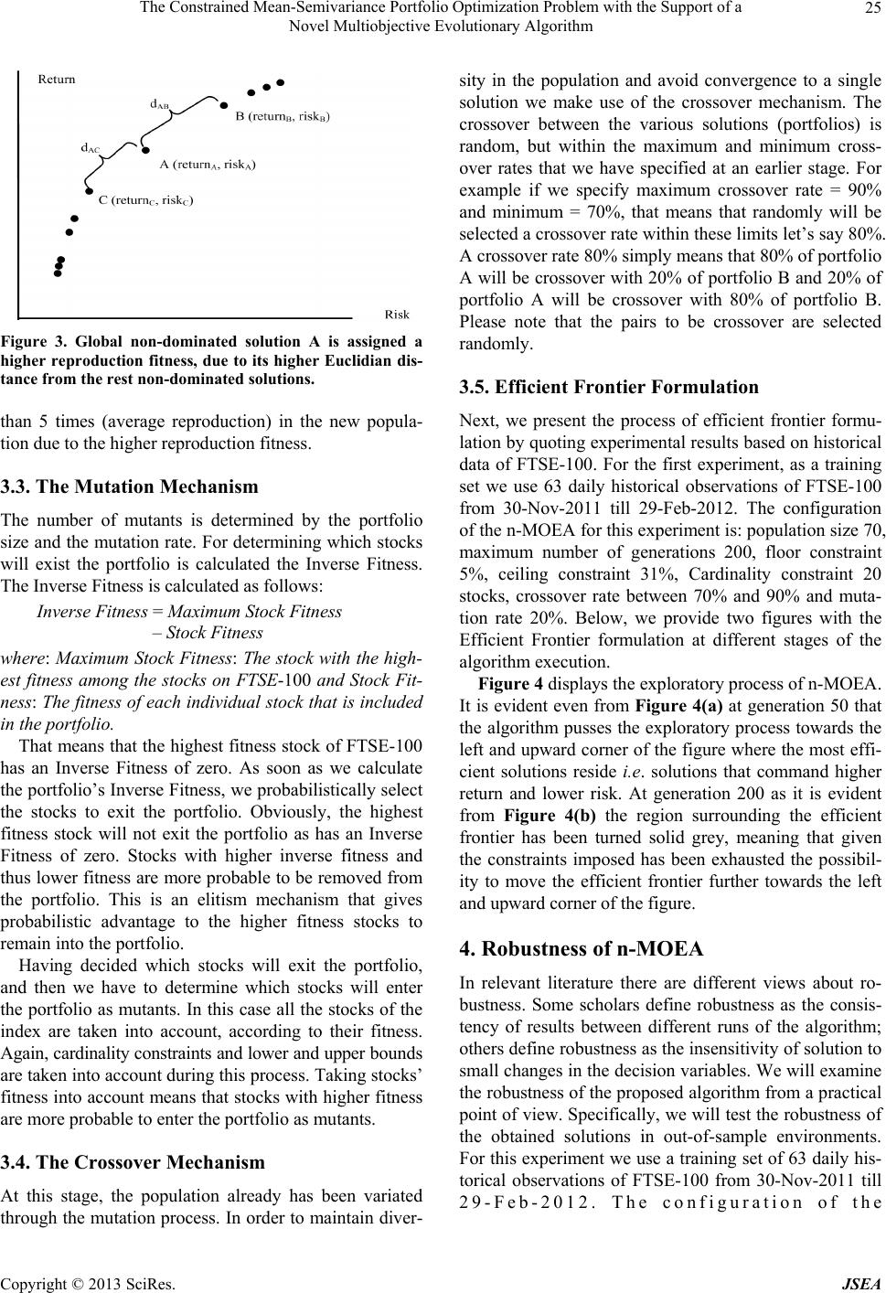
Figure 3. Global non-dominated solution A is assigned a
higher reproduction fitness, due to its higher Euclidian dis-
tance from the rest non-dominated solutions.
than 5 times (average reproduction) in the new popula-
tion due to the higher reproduction fitness.
3.3. The Mutation Mechanism
The number of mutants is determined by the portfolio
size and the mutation rate. For determining which stocks
will exist the portfolio is calculated the Inverse Fitness.
The Inverse Fitness is calculated as follows:
Inverse Fitness = Maximum Stock Fitness
– Stock Fitness
where: Maximum Stock Fitness: The stock with the high-
est fitness among the stocks on FTSE-100 and Stock Fit-
ness: The fitness of each individual stock that is included
in the portfolio.
That means that the highest fitness stock of FTSE-100
has an Inverse Fitness of zero. As soon as we calculate
the portfolio’s Inverse Fitness, we probabilistically select
the stocks to exit the portfolio. Obviously, the highest
fitness stock will not exit the portfolio as has an Inverse
Fitness of zero. Stocks with higher inverse fitness and
thus lower fitness are more probable to be removed from
the portfolio. This is an elitism mechanism that gives
probabilistic advantage to the higher fitness stocks to
remain into the portfolio.
Having decided which stocks will exit the portfolio,
and then we have to determine which stocks will enter
the portfolio as mutants. In this case all the stocks of the
index are taken into account, according to their fitness.
Again, cardinality constraints and lower and upper b ou nd s
are taken into account during this process. Taking stocks’
fitness into account means that stocks with higher fitness
are more probable to enter the portfolio as mutants.
3.4. The Crossover Mechanism
At this stage, the population already has been variated
through the mutation process. In order to maintain diver-
sity in the population and avoid convergence to a single
solution we make use of the crossover mechanism. The
crossover between the various solutions (portfolios) is
random, but within the maximum and minimum cross-
over rates that we have specified at an earlier stage. For
example if we specify maximum crossover rate = 90%
and minimum = 70%, that means that randomly will be
selected a crossover rate within these limits let’s say 80%.
A crossover rate 80% simply means that 80% of portfolio
A will be crossover with 20% of portfolio B and 20% of
portfolio A will be crossover with 80% of portfolio B.
Please note that the pairs to be crossover are selected
randomly.
3.5. Efficient Frontier Formulation
Next, we present the process of efficient frontier formu-
lation by quoting experimental results based on historical
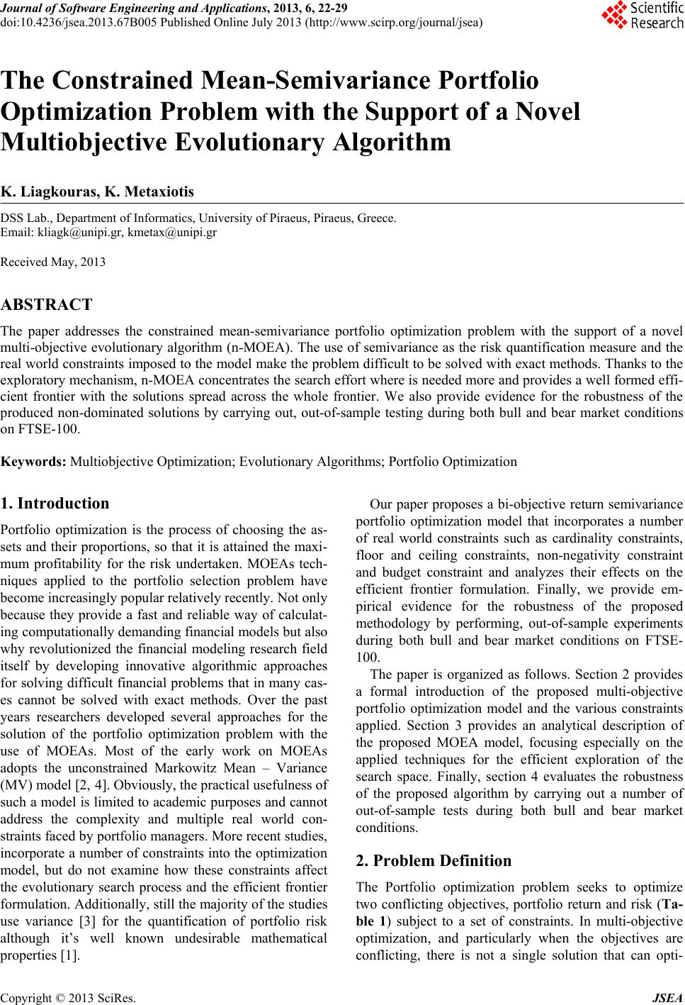
data of FTSE-100. For the first experiment, as a training
set we use 63 daily historical observations of FTSE-100
from 30-Nov-2011 till 29-Feb-2012. The configuration
of the n-MOEA for this experiment is: population size 70,
maximum number of generations 200, floor constraint
5%, ceiling constraint 31%, Cardinality constraint 20
stocks, crossover rate between 70% and 90% and muta-
tion rate 20%. Below, we provide two figures with the
Efficient Frontier formulation at different stages of the
algorithm execution.
Figure 4 displays the exploratory process of n-MOEA.
It is evident even from Figure 4(a) at generation 50 that
the algorithm pusses the exploratory process towards the
left and upward corn er of the figure where the most effi-
cient solutions reside i.e. solutions that command higher
return and lower risk. At generation 200 as it is evident
from Figure 4(b) the region surrounding the efficient
frontier has been turned solid grey, meaning that given
the constraints imposed has been exhausted the possibil-
ity to move the efficient frontier further towards the left
and upward corner of the figure.
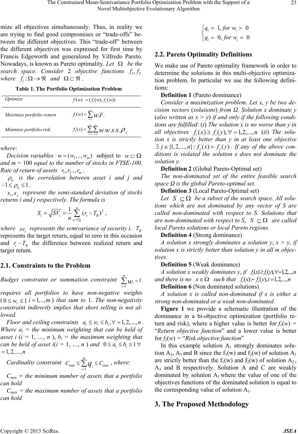
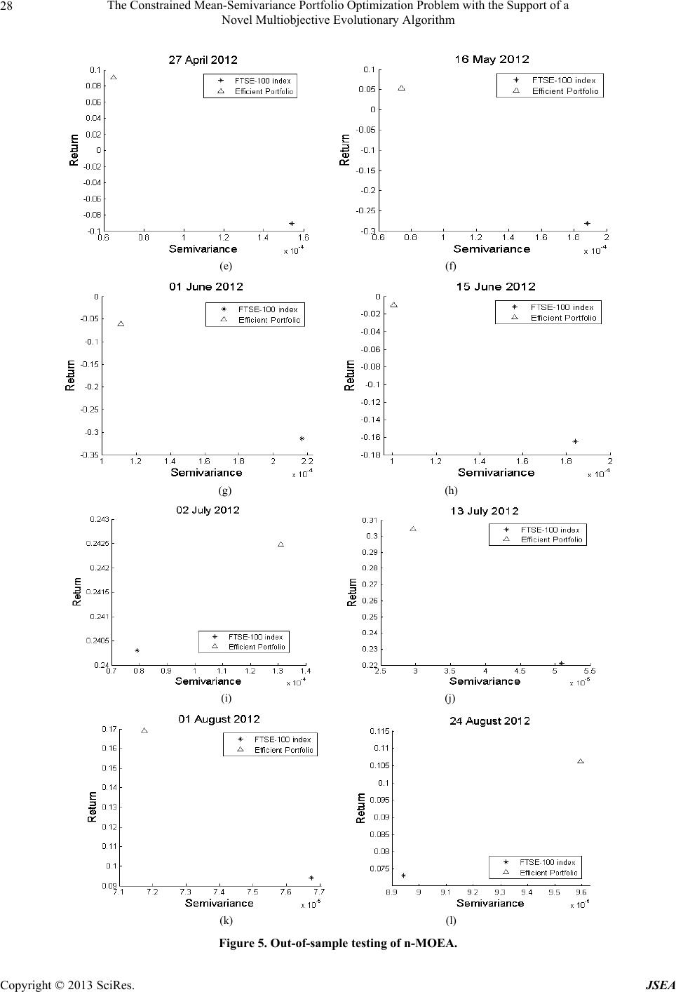
4. Robustness of n-MOEA
In relevant literature there are different views about ro-
bustness. Some scholars define robustness as the consis-
tency of results between different runs of the algorithm;
others define robustness as the insensitivity of solution to
small changes in the decision variables. We will examine
the robustness of the proposed algorithm from a practical
point of view. Specifically, we will test the robustness of
the obtained solutions in out-of-sample environments.
For this experiment we use a training set of 63 daily his-
torical observations of FTSE-100 from 30-Nov-2011 till
29-Feb-2012. The configuration of the

Current Distortion Evaluation in Traction 4Q Constant Switching Frequency Converters 26
sv
(a)
sv
(b)
Figure 4. Exploratory process of n-MOEA.
n-MOEA for this experiment is: population size 70,
maximum number of generations 200, floor constraint
5%, ceiling constraint 31%, Cardinality constraint 20
stocks, crossover rate between 70% and 90% and muta-
tion rate 20%. The objective of this experiment is to test
whether the non-dominated solutions emerged during the
in-sample testing remain robust in out-of-sample testing.
It is well known that portfolio managers of large funds in
order to succeed satisfactory diversification and achieve
better returns, keep in their portfolios stocks from every
component of FTSE-100 index. However, this strategy
can be followed only by big players and is associated
with high administrative costs.
The purpose of this experiment is to find out if it is
possible to outperform the FTSE-100 index performance
by formulating an efficient portfolio that consist a small
chunk of the whole index. If the experiment is successful
it will mean that we are able to command combinations
of higher return and lower risk than the FTSE-100 index
with just a small proportion of the investment require-
ment and administrative costs associated with index
portfolios. Please notice that during the out-of-sample

The Constrained Mean-Semivariance Portfolio Optimization Problem with the Support of a
Novel Multiobjective Evolutionary Algorithm 27
testing period of six months (March to August 2012) we
do not rebalance our efficient portfolio. Table 2 presents
the Efficient portfolio and the corresponding stocks and
weights as these emerged during the optimization process.
For carrying out the test we separate the out-of-sample
period of six months into twelve intervals. For the calcu-
lation of return and risk have been taken into account 30
observations, with ending observation the one that appear
on the title of each graph of Figure 5. Thus, for example
in Figure 5(e) for the calculation of return and risk
of both Efficient portfolio and FTSE-100 index alike, are
Table 2. The Efficient Portfolio and the corresponding
stocks and weights
Efficient Portfolio
stock weight
ABF.L 29.81%
BNZL.L 30.64%
GFS.L 8.92%
SN.L 11.27%
DGE.L 19.36%
taken into account 30 observations, with last observation
the 27-April-2012 (same as the title of the graph) and
first observation if we count 30 trading days backwards
the 15-March-2012. From the Figure 5 it is evident that
Efficient portfolio strongly dominates FTSE-100 index
return and risk combinations in 9 out of 12 cases. Even
six months after its formulation, the efficient portfolio,
strongly dominates FTSE- 100 index return and risk as it
appears clearly in Figure 5(k). In only, 3 situations
(Figures 5(b), (i) and (l)) efficient portfolio and
FTSE-100 index are non-dominated which means that
efficient solution is not strictly or weakly better than
FTSE-100 index. It is worth mentioning that in none
situation FTSE-100 index performance dominates effi-
cient portfolio performance during this six months
out-of-sample testing period. This is a strong indication
of the robustness of the solution produced by the
n-MOEA. Finally, we should highlight that the six
months out-of-sample testing period includes both bull
and bear market periods and as it is evident from Figure
5, the n-MOEA Efficient portfolio proved robust in both
upward and downward market conditions.
(a) (b)
(c) (d)

The Constrained Mean-Semivariance Portfolio Optimization Problem with the Support of a
Novel Multiobjective Evolutionary Algorithm
28
(e) (f)
(g) (h)
(i) (j)
(k) (l)
Figure 5. Out-of-sample testing of n-MOEA.

The Constrained Mean-Semivariance Portfolio Optimization Problem with the Support of a
Novel Multiobjective Evolutionary Algorithm
29
5. Conclusions
In this paper, we have proposed a novel MOEA for the
solution of the constrained mean-semivariance portfolio
optimization problem. The algorithm can handle suc-
cessfully downside risk measures like semivariance and
real world constraints and formulate well spread frontiers
thanks to an elitism mechanism applied in the mutation
process that give a reproduction advantage to the higher
fitness stocks, and an exploratory mechanism that uses
the notion that good solutions are more probable to be
found near other non-dominated solutions. At the same
time another mechanism calculates the Euclidian dis-
tance between the various non-dominated solutions in
order to assign reproduction fitness. That way, we safe-
guard that the exploratory effort is concentrated where is
needed more and the solutions are spread across the en-
tire frontier. Also, the crossover process enhances the
population diversity, by combining randomly two
non-dominated solutions to produce two new off-springs.
The robustness of the proposed algorithm is verified for
short and mid-term by carrying out a number of
out-of-sample tests during both bull and bear market
conditions on FTSE-100.
REFERENCES
[1] P. Artzner, F. Delbaen, J. Eber and D. Heath, “Coherent
measures of risk. Mathematical Finance,”Mathematical
Finance, Vol. 9, No.3, pp.203–228.
doi:10.1111/1467-9965.00068
[2] H. M. Markowitz, “Foundations of Portfolio Theory,”
Journal of Finance, Vol.46, No. 2, 1991, pp.469-477.
doi:10.1111/j.1540-6261.1991.tb02669.x
[3] K. Metaxiotis and K. Liagkouras, “Multiobjective Evolu-
tionary Algorithms for Portfolio Management: A com-
prehensive Literature Review,” Expert Systems with Ap-
plications 39, Vol.39, No. 14, 2012, pp.11685–11698.
doi:10.1016/j.eswa.2012.04.053
[4] F. Pasiouras, S. Tanna and C. Zopounidis, “The Impact of
Banking Regulations on Bank’s Cost and Profit Effi-
ciency: Cross country Evidence,” International Review of
Financial Analysis, Vol. 18, No. 5, 2009, 294 - 302.
doi:10.1016/j.irfa.2009.07.003