Engineering, 2013, 5, 27-31
http://dx.doi.org/10.4236/eng.2013.510B006 Published Online October 2013 (http://www.scirp.org/journal/eng)
Compensation of Finite Bandwidth Effect by Using an
Optimal Filter in Photoacoustic Imaging*
Chen Zhang, Yan Zhang, Yuanyuan Wang
Department of Electronic Engineering, Fudan University, Shanghai, China
Received September 2012
ABSTRACT
Most existing reconstruction algorithms for photoacoustic imaging (PAI) assume that transducers used to receive ultra-
sound signals have infinite bandwidth. When transducers with finite bandwidth are used, this assumption may result in
reduction of the imaging contrast and distortions of reconstructed images. In this paper, we propo s e a novel method to
compensate the finite bandwidth effect in PAI by using an optimal filter in the Fourier domain. Simulation results
demonstrate that the use of this method can improve the contrast of the reconstruc ted images with finite-bandwidth ul-
trasound transducers.
Keywords: Photoacoustic Tomography; Finite Bandwidth Effect; Optimal Filter
1. Introduction
Photoacoustic imaging (PAI) is a promising medical im-
aging modality that has great potential for a wide ra nge
of clinical imaging applications [1,2]. PAI is a hybrid
imaging method that combines the high contrast of opti-
cal imaging and the high spatial resolution of ultrasonic
imaging. Due to its noninvasive nature, it is a technique
which is harmless for the human body [2].
In PAI, pulsed laser energy is delivered to an object
and the thermoacoustic effect will result in the generation
of the ultr asound wav e. Ultrasound signals are t hen de-
tected by the scanning ultrasound transducers. With these
received signals, an image reconstruc tion algorithm is
used to reconstruct the image of an object’s optical ab-
sorption distribution.
A variety of research has been done on the f ield of
image reconstr uction algorithms [3-10]. Most of these
algorithms are based on th e assumption that infinite-
bandwidth transducers are employed to receive ultra-
sound signals. Without incorporating characteristics of
ultrasound transducers in the imaging reconstruction
model, the resolution and the contrast of reconstructed
images will be significantly degraded. Several imaging
models have been established to incorporate physical
characteristics of ultrasound transducers [11,12]. How-
ever, none of them takes the finite bandwidth effect of
ultrasound tr ansd uc e r s into account.
In this paper, we propose a novel image reconstruction
algorithm that incorporates the finite ba ndwidth ch arac-
teristics of ultrasound tr ansducers. An optimal filter is
designed to deconvolve the transducer’s impulse re-
sponse of the finite bandwidth at each imaging point.
Through the numerical simulation, the proposed algo-
rithm is compared to those recons truction algorithms
assuming finite-bandwidth ultrasound transducers.
2. Theory and Method
2.1. Basic Principles of PAI
In this study, we intend to solve the problem with 2D
circular-scanning PAI mode. In this mode, a short pulse
is used to illuminate the imaging object from the top, and
an ultrasoun d transducer is circularly sc anned a rou nd the
object to record the ultr a s ound data. The relation between
the optical absorption distribution and the gen erated ul-
trasonic waves can be deduced as [3]:
2
2
22
1 (,)()
(,) ()
p
p tIt
pt A
Ct ct
β ∂∂
∇−=− ∂
∂
r
rr
, (1)
where c is the speed of sound,
β
is the volume thermal
expansion coefficient and Cp is the specific heat. A(r) is
the unknown absorption distribution and I(t) is the illu-
mination function. A solution to this equation can be
obtained by the use of Green’s function. In the case of
illumination with a short pulse, p(r, t) can be deduced as:
0
2
0'
( ')
( ,)'
4ct
p
A
pt d
Ct t
β
π
−=
∂
=∂∫∫rr
r
rr

(2)
Equation (2) represent s an idealized imaging model for
*Natural Science Foundation of China (
No. 61271071 and No.
11228411) and Specialized Research Fund forthe Doctoral
Program of
Higher Edu cation of China (No. 201 1 0 071110017).

C. ZHANG ET AL.
28
PAI. The image reconstruction problem is to determine
an estimate of A(r) from the know ledge of p(r, t). A va-
riety of image reconstruction algorithms [3-10] ha s been
developed for the inversion of (2). However, those algo-
rithms neglect the response characteristics of the trans-
ducer. Therefore they may produce significant image
blurring and low contrast in the reconstructed images.
2.2. Finite Bandwidth Effect of a Transducer
Most of PAI reconstruction algorithms are based on the
assumption that the bandwidth of ultrasonic transducers
which are employed to receive signals is infinite. How-
ever, actual ultrasound transducer s are all with the finite
bandwidth. The finite bandwidth effect of transducers
can be expressed as a convolution of received signals and
an impulse respon se. The actual projection data can be
expressed as:
00
( ,)( ,)(,)
ideal
prtprt hrt= ∗
, (3)
where the pideal(r0,t) is the idealized projection data based
on the assumption that the transducers have the infinite
bandwidth, p(r0,t) is the actual projection data obtained
by the transducers, h(r0,t) is the impulse response of the
transducer related to its bandwidth, * denotes a one-di-
mensional temporal convolution.
Figure 1 compares ultrasonic signals obtained by an
idealized transducer and a finite-bandwidth transducer.
Ultrasonic signals are excited by a point optical absorber.
Figure 1 illustrated that the finite-bandwidth effect may
cause the reduction of the signal density and the convo-
lutional noise. These are major reasons of image blurr ing
and low contrast in reconstructed images if image recon-
struction algorithms fail to take the finite-bandwidth ef-
fect into account.
Figure 1. A comparison between ultrasou nd signals obtaine d
by an idealized transducer and a finite-bandwidth trans-
ducer.
2.3. Compensating for the Finite Bandwidth
Effect
Based on (3), the purpos e of compensation for the finite
bandwidth effect is to obtain the pideal(r0,t). As the re-
ceived signals are non-stationary signals, we use the
short time Fourier transform (STFT) to transform the
data into the Fourier domain. Here we take the additive
noise into account. Equation (3) is transformed as:
00
(,)(,) (,)
ideal
PrP rHre ω ωω = ⋅+
(4)
where e is the additive noise, H(r, ω)is the bandwidth of
the transducer, P(r0, ω) and Pideal(r0, ω)is the Fourier
spectrum of the actual projection data and the idealized
data.
An optimal filter T can be derived to obtain received
signals wher e th e finite bandwidth effect is compensated.
00
(,) (,)
ideal
PrTPr ωω = ⋅
(5)
In this study, this optimal filter T is designed to mi-
nimize the error between P(r0, ω) and Pideal(r0, ω). At the
same time, th e optimal filter should have good robustness
against the additive noise. We can easily get the band-
width characteristics of a transducer from its data sheet
or from the physical meansurement experiment. In the
Fourier domain, its distribution function is Gaussian. The
optimal filter T can be found:
2
1 /(1/)T φ = +∆
, (6)
where
ϕ
is a parameter determine the noise suppres-
sion effect and
∆
a Gaussian kernel function which can
be expressed as:
2
()
2
1
2
t
e
µ
σ
σπ
−
−
∆=
. (7)
Here μ is the mean of the function, σ is the variance of
the function. Both of those parameters can be obtained
from the bandwidth characteristics of the transducer.
Once we obtained the actual projection data, we can
reconstruct the image with the compensated data.
3. Results and Discussion
Simulations are performed to ev alu ate the efficacy of this
method on the improvement of resolution and contrast of
the reconstructed image. The comparison are made
among this method and those reconstruction algorithms
assuming finite-bandwidth ultrasound transducers. All
simulations are done using the K-wave toolbox [13,14]
of MATLAB.
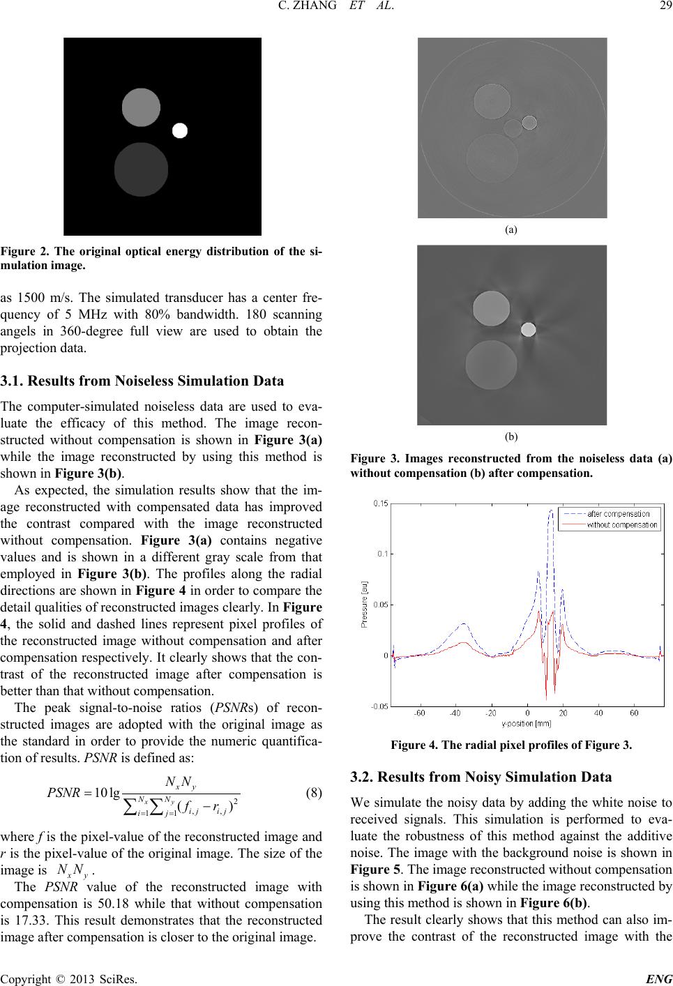
In this simulation, three optical absorbers with differ-
ent radius and optical absorption density are located in
the test image. Its original optical energy distribution is
showed in Figure 2. We set the radius of scanning circle
as 250 pixels and assume the speed of sound consistent

C. ZHANG ET AL.
29
Figure 2. The original optical energy distribution of the si-
mulation image.
as 1500 m/s. The simulated transducer has a center fre-
quency of 5 MHz with 80% bandwidth. 180 scanning
angels in 360-degree full view are used to obtain the
projection data.
3.1. Results from Noiseless Simulation Data
The computer-simulated noiseless data are used to eva-
luate the efficacy of this method. The image recon-
structed without compensation is shown in Figure 3(a)
while the image reconstructed by using this method is
shown in Figure 3(b).
As expected, the simulation results show that the im-
age reconstructed with compensated data has improved
the contrast compared with the image reconstructed
without compensation. Figure 3(a) contains negative
values and is shown in a different gray scale from that
employed in Figure 3(b). The profiles along the radial
directions are shown in Figure 4 in order to compare the
detail qualities of reconstructed images clearly. In Figure
4, the solid and dashed lines represent pixel profiles of
the reconstructed image without compensation and after
compensation respectively. It clearly shows that the con-
trast of the reconstructed image after compensation is
better than that without compensation.
The peak signal-to-noise ratios (PSNRs) of recon-
structed images are adop ted with the original image as
the standard in order to provide the numeric quantifica-
tion of results. PSNR is defined as:
2
,,
11
10lg ()
xy
xy
NN
ij ij
ij
NN
PSNR fr
= =
=−
∑∑
(8)
where f is the pixel-value of the reconstructed image and
r is the pixel-value of the original image. The size of the
image is
xy
NN
.
The PSN R value of the reconstructed image with
compensation is 50.18 while tha t without compensation
is 17.33. This result demonstrates that the reconstructed
image after compensation is closer to the original image.
(a)
(b)
Figure 3. Images reconstructed from the noiseless data (a)
without compensation ( b) after co m pe nsation.
Figure 4. The radial pixel profiles of Figure 3.
3.2. Results from Noisy Simulation Data
We simulate the noisy data by adding the white noise to
received signals. This simulation is performed to eva-
luate the robustness of this method against the additive
noise. The image with the back ground noise is shown in
Figure 5. The image reconstructed without compensation
is shown in Figure 6(a) while the image reconstructed by
using this method is shown in Figure 6(b).
The result clearly shows that this method can also im-
prove the contrast of the reconstructed image with the

C. ZHANG ET AL.
30
Figure 5. The simulation image with the background noise .
(a)
(b)
Figure 6. The images reconstructed from the noisy data (a)
without compensation (b)after co m pe nsation.
noisy data. This seems to be a robust algorithm. The pro-
files along the radial directions are shown in Figure 7. In
Figure 7, the solid and dashed lines represent the pixel
profiles of the reconstructed image without compensation
and after compensation respectively. It clearly shows that
the contrast of the reconstructed image after compensa-
tion is better than that without compensation. It is also
seen that the density of the noise is weaker than that
without compensation. Through this simulation, the re-
sult shows that this method can reconstruct images with
Figure 7. The radical pixel profiles of Figure 6.
lower noise levels, meanwhile the algorithm is robust.
4. Conclusion
In this paper, we propose a method to compensate the
finite bandwidth effect of the ultrasou nd transducer. It is
seen from simulation studies that the proposed method
has good robustn es s and can effectively improve the im-
age contrast for PAI with finite-bandwidth transducers.
REFERENCES
[1] L. V. Wang, “Tutorial on Photoacoustic Microscopy and
Computed Tomography,” I EEE Journal of Selected Top-
ics Quantum Electronics, Vol. 14, No. 1, 2008, pp. 171-
179. http://dx.doi.org/10.1109/JSTQE.2007.913398
[2] C. Li and L. V. Wang, “Photoacoustic Tomography and
Sensing in Biomedicine,” Physics in Medicine and Biol-
ogy, Vol. 54, No. 19, 2009, pp. R59-R97.
http://dx.doi.org/10.1088/0031-9155/54/19/R01
[3] M. Xu and L. V. Wang, “Universal Back-Projection Al-
gorithm for Photacoustic Computed Tomography,” Phys-
ical Review E, Vol. 71, No. 1, Article ID: 016706.
http://dx.doi.org/10.1103/PhysRevE.71.016706
[4] P. Burgholzer, J. Bauer-Marschallinger, H. Grun, M.
Haltmeier and G. Paltauf, “Temporal Back-Projection
Algorithms for Photoacoustic Tomography with Integrat-
ing Line Det ectors,” Inverse Problems, Vol. 23, No. 6,
2007, pp. S65-S80.
http://dx.doi.org/10.1088/0266-5611/23/6/S06
[5] M. Xu, Y. Xu and L. V. Wang, “Time-Doma in Recon-
struction Algorithms and Numerical Simulations for Ther-
moacoustic Tomography in Various Geometries,” IEEE
Transactions on Biomedical Engineering, Vol. 50, No. 9,
2003, pp. 1086-1099.
http://dx.doi.org/10.1109/TBME.2003.816081
[6] Y. Xu, D. Feng and L. V.Wang, “Exact Frequency-Do-
main Reconstruction for Thermoacoustic Tomography: I.
Planar Geometry,” IEEE Transactions on Medical Imag-

C. ZHANG ET AL.
31
ing, Vol. 21, No. 7, 2002, pp. 823-828.
http://dx.doi.org/10.1109/TMI.2002.801172
[7] L. A. Kunyansky, “Explicit Inversion Formulae for the
Spherical Mean Radon Transform,” Inverse Proble ms,
Vol. 23, 2007, pp. 373-383.
http://dx.doi.org/10.1088/0266-5611/23/1/021
[8] M. A. Anastasio, J. Zhang, X. Pan, Y. Zou, G. Keng and
L. V. Wang, “Half-Time Image Reconstruction in Ther-
moacoustic Tomography,” IEEE Transactions on Medi-
cal Imaging, Vol. 24, No. 2, 2005, pp. 199-210.
http://dx.doi.org/10.1109/TMI.2004.839682
[9] P. Ephrat, L. Keenliside, A. Seabrook, F. S. Prato and J. J.
L. Carson, “Three-Dimensional Photoacoustic Imaging
by Sparse-Arra y Detection and Iterative Image Recon-
struction,” Journal of Biomedical Optics, Vol. 13, No. 5,
2008. http://dx.doi.org/10.1121/1.1501898
[10] G. Paltauf, J. A. Viator, S. A. Prahl and S. L. Jacques,
“Iterative Reconstructional Gorithm for Optoacoustic Im-
aging,” Journal of the Acoustical Society of America, Vol.
112, No. 4, 2002, pp. 1536-1544.
http://dx.doi.org/10.1121/1.1501898
[11] K. Wang, S. A. Ermilov, R. Su, H. Brecht, A. A.
Oraevsky and M. A. Anastasio, “An Imaging Model In-
corporating Ultrasonic Tranducer Properties for Three-
Dimensional Optoacoustic Tomography,” IEEE Transac-
tions on Medical Imaging, Vol. 30, No. 2, 2011, pp. 203-
213. http://dx.doi.org/10.1109/TMI.2010.2072514
[12] M. Li, Y. Tseng and C. Cheng, “Model-Based Correction
of Finite Aperture Effect in Photoacoustic Tomography,”
Optics Express, Vol. 18, No. 25, 2010.
http://dx.doi.org/10.1364/OE.18.026285
[13] B. T. Cox, S. Kar a, S. R. Arridge and P. C. Beard,
“k-Space Propagation Models for Acoust ically Heteroge-
neous Me dia: Application to Biomedical Photoacoustics,”
Journal of the Acoustical Society of America, Vol. 121,
No. 6, 2007, pp. 3453-3464.
http://dx.doi.org/10.1121/1.2717409
[14] B. E. Treeby and B. T. Cox, “k-Wave: MATLAB Tool-
box for the Simulation and Reconstruction of Photoac-
oustic Wave Fields,” Journal of Biomedical Optics, Vol.
15, No. 2, 2010. http://dx.doi.org/10.1117/1.3360308