 Journal of Applied Mathematics and Physics, 2013, 1, 58-64 Published Online November 2013 (http://www.scirp.org/journal/jamp) http://dx.doi.org/10.4236/jamp.2013.15009 Open Access JAMP Hermite Matrix Polynomial Collocation Method for Linear Complex Differential Equations and Some Comparisons Mina Bagherpoorfard, Fahime Akhavan Ghassabzade* Department of Mathematics, Islamic Azad University, Fasa Branch, Fasa, Iran Email: mi.bagherpoorfard@um.ac.ir, *akhavan_gh@yahoo.com Received August 20, 2013; revised September 25, 2013; accepted October 1, 2013 Copyright © 2013 Mina Bagherpoorfard, Fahime Akhavan Ghassabzade. This is an open access article distributed under the Creative Commons Attribution License, which permits unrestricted use, distribution, and reproduction in any medium, provided the original work is properly cited. ABSTRACT In this paper, we introduce a Hermite operational matrix collocation method for solving higher-order linear complex differential equations in rectangular or elliptic domains. We show that based on a linear algebra theorem, the use of dif- ferent polynomials such as Hermite, Bessel and Taylor in polynomial collocation methods for solving differential equa- tions leads to an equal solution, and the difference in the numerical results arises from the difference in the coefficient matrix of final linear systems of equations. Some numerical examples will also be given. Keywords: Approximate Solution; Collocation Methods; Complex Differential Equations; Hermite Polynomials; Operational Matrix 1. Introduction Complex differential equations and their solutions play a major role in science and engineering. A physical event can be modeled by complex differential equations. Since a few of these equations cannot be solved explic- itly, it is often necessary to resort to approximation and numerical techniques. In recent years, the studies on complex differential equations were developed very rap- idly [1-6]. Since 1994, matrix polynomial collocation approaches such as Taylor and Bessel matrix collocation methods have been used by Sezer and colleagues [7-11] to solve the complex linear differential equations. The present work contains two main parts, in the first part, we use Hermite matrix collocation method to find the approximate solution of higher-order linear complex differential equations of the following form. 0, k nk k zf gz (1) which is a generalized case of the complex differential equations given in [5,6], with themixed conditions 1 00 ;0,1,, Jm k rkj r kj afr m 1 (2) in the following rectangular domain ,, ,,,,,DzxiyzcaxbcydabcdR , (3) or elliptic domain ,, cos, sin, 02, ,, Dzxiyzcxayb axabybab R (4) In the second part, we will study the effect of using different polynomial classes on the matrix polynomial methods. The outline of this paper is as follows. In Section 2, we briefly introduce Hermite polynomial and describe de- tails of using these polynomials in matrix polynomial collocation method. Section 3 focuses on the comparison of matrix collocation methods when different polynomi- als are used. We present the results of numerical experi- ments in Section 4. Finally, conclusions are drawn in Section 5. 2. Hermite Matrix Polynomial Collocation Method In this section, we describe the matrix form of Hermite polynomials and Hermite collocation Method for com- plex differential equations. Our aim is to find an ap- *Corresponding author.  M. BAGHERPOORFARD, F. A. GHASSABZADE 59 proximate solution of (1) defined by a truncated Hermite series form 0, Nnn n N zaHzHz A (5) where 01 N HzHzH zHz such that ,0,1,, n zn N are the Hermite polynomials de- fined by 0 2 2 2 !1 !2! nj jnj n N j Hz nz jn j , where 2 n N if n is even and 1 2 n N if n is odd and . It is well known [12] that the relation between the powers T 12 N Aaa a 2 2 20 2! ;0 1, !2 ! 2 n n nn r nHz Zz rn n' (6) and 21 21 21 0 21! ;0 1 !(21)! 2 n r n nn nHz Zz rn n' (7) By using the expression (6) and (7) and taking 0,1,,nN we find the corresponding matrix relation as follows T T zMHz, and z and Hermite poly- nomials is T zHzM, (8) where 2 1N zzzz , for odd N 1 2 11 24 31 48 !! 11 2!1!2 1!3! 22 100 0 000 00 00 00 NN NN NN M 0 0 0 0 0 and for even N 10 0 00 000 00 00 1 2 11 24 31 48 !! 20!! 2!0!2 1!2! 22 00 N NN NN NN N M 0 0 0 !N Then, by taking into account (5), we obtain T 1 HzZz M and we can replace series (6) in the matrix form T 1 N zHzAZzM A . (9) Furthermore, the relation between the matrix z and its derivative 1 z is (1) T zZzB, (10) where T 010 0 002 0 000 000 0 B N And Open Access JAMP  M. BAGHERPOORFARD, F. A. GHASSABZADE 60 0 T 100 0 010 0 000 1 B From the matrix Equation (10), we get the following relations: 2 21 TT 3 32 TT 1TT , , . k kk ZzZzBZzB ZzZzBZzB ZzZ zBZzB (11) By using relations (9) and (11), we have a recurrence relation in what follows T 1T k kk N T 1 zZzMAZzBM A . (12) For the collocation points , the matrix relation (12) becomes pq zz T T1 ; ,0,1,, . k pq pq k N zZzBMApq N N (13) For one can write the relation (13) in the following form 0,1, ,p T T1 00 T T1 11 T T1 , , . k qq k qq k N k N k N k Nq Nq zZzBMA zZzBMA zZzBM A or briefly 0 10,1,, , k Nq k kNq q k NNq q fz fz f fz N (14) where 2 000 0 2 111 1 2 1 1 1 N qqq q N qqq q q N qNqNq Nq Zz zzz Zz zz z Z zzz Zz Moreover, substituting the collocation points into Eq- uation (3), we have 0;,0,1,, . k kpqN m pq pq kPzfzgzpqN (15) By means of the expressions (13) and (14), we acquire the fundamental matrix equation T T1 00 0 k kq qq k m qq NN PZ BMAG (16) In which 0 1 00 00 00 kq kq kq kNq pz pz P pz and ,,, qqqNq Ggzgz gzT 01 . With the aid of relation (12), we can obtain the corresponding matrix form due to the condition (4) as follows T T1 00 0, 1;,,1, k rk j k m j J r aZB M mAr (17) where 2 1N jjj Zj . Briefly, the system of the matrix Equation (17) can be written in the matrix form or ; rr r UAu r , (18) where T T1 00 01 0;,1,, mk rk j kj rN J rr aZBM uur mu 1, We can write Equation (16) in the form WA G, (19) such that T T1 00 ; k kq m q q st k kPZ BMWw 1,,,,0, tN and 0 1 0q q N N GG , where Gq is defined in (16). The augmented matrix of Equation (19) becomes ;;; ,0,1, st s WGw gstN,. (20) The augmented matrix of Equation (18) corresponds to 01 ; rrrrrN r Uuuu; , where Ur is defined in (18). Consequently, to find the unknown Hermite coeffi- cients an, 0,1, ,nN related to approximate solution of the problem consisting of Equation (3) and condition (4), we replace the matrices (20) by the last m rows of Open Access JAMP  M. BAGHERPOORFARD, F. A. GHASSABZADE 61 the augmented matrix (19). Hence, we have a new aug- mented matrix , where * WA G ** 00 01 10 11 20 21 01 00 01 10 11 20 10 11 21 Nm Nm mm ww ww ww ww uu uu uu uu * 020 0 1 22 2 2 020 0 121 1 2 12 12 1 2 22 2 11 ; N NmNmN Nm N N N N m Nm N m WG ww g ww g ww g w wg u u u u u u u u (21) If det (W*) ≠ 0 then we can write 1 ** WG ,, , . The unknown Hermite coefficients matrix A, is determined by solving this linear system and 01 aa a n are sub- stituted in Equation (3). Thus, we obtain the Hermite polynomial solution n N Nn zaHz . 3. Comparison of Matrix Polynomial Collocation Methods Theorem3.1. Let 0i be a base for vector space S, then every member s S has a unique representation in the form of linear combination of these vectors. i B k Proof. [13]. Based on the above theorem, if the bases of approxi- mate space in collocation methods are chosen from com- plex polynomials up to degree N, using different bases or choosing of different complex polynomial classes as the base has no effect on the approximate solution, theoretic- cally. This means that if and 0 N nn z 0 N nn z be two different bases according to the uniqueness repre- sentation, then approximate solution of (1) can be written 00 . NN n nn nn Nn za 0,1,,n za z N For this reason when we use different polynomials (such as Taylor, Bessel, Hermite, etc.) in polynomial Collocation methods one expects the equal results ob- tained. In the numerical implementation, to determine coef- ficients an, in (5), we should solve a sys- tem of equations in the form of WF = G and properties of matrix W is directly depended on choosing the base. So different bases result different matrix W with different properties. Some of these properties such as condition number has the direct influence on solution’s accuracy. In addition CPU time for solving these systems differs for different bases. Hence, different polynomial bases can cause solutions with different accuracy. Our experiences show that when we use different po- lynomial classes in matrix polynomial collocation meth- ods, there is negligible difference among approximated solutions. In Section 4, we compare this matter for sev- eral examples by using Taylor, Bessel and Hermite po- lynomials. 4. Numerical Examples Several numerical examples are studied in this section to illustrate the accuracy and efficiently properties of Taylor, Bessel and Hermite collocation method. In this paper, collocation points in the rectangular domain (3) are de- fined by qp zxiy q , such that ,, ;,0,1, , pq q ba dc, p apycqax NN cy dpqN b and in the elliptic domain (4) are defined by , pqpqpqpq pq zxiyxy D , cos , pq a pq NN sin , pq b yp NN q such that ,0,1,,pq N ; , 02q 0 0, 0 00 zz q Examples show that the difference among collocation methods based on these polynomials is negligible. All of them are performed on a computer using programs writ- ten in MATLAB 2011a. In this regard, we have reported in the Tables the value of absolute error function . N ezfNfz N at the selected points of the domain. 4.1. Example 1 As the first example, [10], we consider the linear second order complex differential equation 2 2 126 5cos2 sin, zfz zfzfz zzzz with 1 0,0 2 ff 0 and exact solution 2 31 cos 22 zz z on elliptic domain with 1 1, 2 ab and . Absolute errors are listed in able 1. T Open Access JAMP  M. BAGHERPOORFARD, F. A. GHASSABZADE Open Access JAMP 62 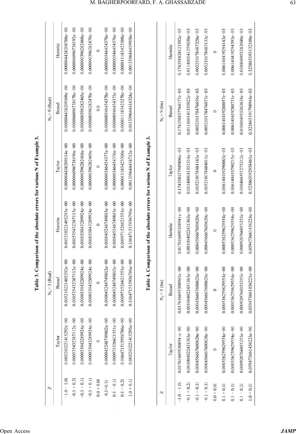 M. BAGHERPOORFARD, F. A. GHASSABZADE 63 Open Access JAMP  M. BAGHERPOORFARD, F. A. GHASSABZADE Open Access JAMP 64 4.2. Example 2 In this example, [10], we consider the third order linear complex differential equation 65 432 8e 12e30e 19e9e0, zz zzz fz fz fz with the condition , , 2 0ef 2 03ef 2 014ef and exact solution 2 ee z fz in el- liptic domain with a=1, 1 2 b and . Absolute errors of the obtain solutions are given in Table 2. 4.3. Example 3 The last example, [11] is the second order complex dif- ferential equation ee z zzfz z , with the initial conditions 01f, 0f1 . The exact solution is e fz on rectangular domain with a = −1, b = 1, c = −1, d = 1. Absolute errors are listed in Tables 3 and 4. 5. Conclusion In this article, approximate solutions which can be ob- tained by different polynomial collocation methods have been compared. Our experiments show that using differ- ent polynomials cannot significantly affect the numerical solutions and the results are similar to each other. REFERENCES [1] G. Barsegian, “Gamma-Lines: On the Geometry of Real and Complex Functions,” Taylor and Frencis, London, 2002. [2] G. Barsegian and D. T. Le, “On a Topological Descrip- tion of Solutions of Complex Differential Equations,” Complex Variables, Vol. 50, No. 7-11, 2005, pp. 307-318. http://dx.doi.org/10.1080/02781070500086743 [3] K. Ishisaki and K. Tohge, “On the Complex Oscillation of Some Linear Differential Equations,” Journal of Ma- thematical Analysis and Applications, Vol. 206, No. 2, 1997, pp. 503-517. http://dx.doi.org/10.1006/jmaa.1997.5247 [4] J. Heittokangas, R. Korhonen and J. Rättyä, “Growth Estimates for Solutions of Linear Complex Differential Equations,” Annales Acade miae Scientiarum Fennicae Ma- thematica, Vol. 29, No. 1, 2004, pp. 233-246. [5] V. A. Prokhorov, “On Best Rational Approximation of Analytic Functions,” Journal of Approximation Theory, Vol. 133, No. 2, 2005, pp. 284-296. http://dx.doi.org/10.1016/j.jat.2004.12.007 [6] V. Andrievskii, “Polynomial Approximation of Analytic Functions on Finite Number of Continua in the Complex Plane,” Journal of Approximation Theory, Vol. 133, No. 2, 2005, pp. 238-244. http://dx.doi.org/10.1016/j.jat.2004.12.016 [7] M. Sezer and M. Güsu, “Approximate Solution of Com- plex Differential Equations for a Rectangular Domain with Taylor Collocation Method,” Applied Mathematics and Computation, Vol. 177, No. 2, 2006, pp. 844-851. http://dx.doi.org/10.1016/j.amc.2005.11.035 [8] M. Güsu and M. Sezer, “Approximate Solution to Linear Complex Differential Equations by a New Approximate Approach,” Applied Mathematics and Computation, Vol. 185, No. 1, 2007, pp. 636-645. http://dx.doi.org/10.1016/j.amc.2006.07.050 [9] M. Sezer and S. Yalcinbas, “A Collocation Method to Solve Higher Order Linear Complex Differential Equa- tions in Rectangular Domains,” Numerical Methods for Partial Differential Equations, Vol. 26, No. 3, 2010, pp. 596-611. [10] M. Sezer, B. Tanay and M. Güsu, “Numerical Solution of a Class of Complex Differential Equations by the Taylor Collocation Method in Elliptic Domains,” Numerical Me- thods for Partial Differential Equations, Vol. 26, No. 5, 2010, pp. 1191-1205. [11] S. Yüzbasi, N. Sahin and M. Sezer, “A Collocation Ap- proach for Solving Linear Complex Differential Equa- tions in Rectangular Domain,” Mathematical Methods in the Applied Sciences, Vol. 35, No. 10, 2012, pp. 1126- 1139. http://dx.doi.org/10.1002/mma.1590 [12] M. Güsu, H. Yalman, Y. Ozturk and M. Sezer, “A New Hermite Collocation Method for Solving Differential Dif- ference Equations,” Applications and Applied Mathemat- ics, Vol. 6, No. 1, 2011, pp. 116-129. [13] K. Haffman and R. Kunze, “Linear Algebra,” 2nd Edition, Prentice-Hall, Upper Saddle River, 1971.
|